Download
1 / 23
230 likes | 397 Views
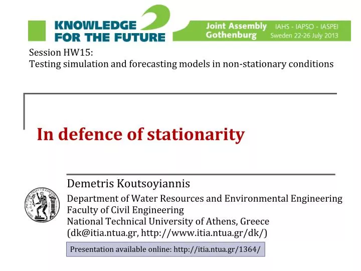
Session HW15: Testing simulation and forecasting models in non-stationary conditions . In defence of stationarity. Demetris Koutsoyiannis

E N D
Session HW15: Testing simulation and forecasting models in non-stationary conditions In defence of stationarity Demetris Koutsoyiannis Department of Water Resources and Environmental Engineering Faculty of Civil EngineeringNational Technical University of Athens, Greece (dk@itia.ntua.gr, http://www.itia.ntua.gr/dk/) Presentation available online: http://itia.ntua.gr/1364/
Premature death, premeditated murder or misinformation? D. Koutsoyiannis, In defence of stationarity
The consensus on the death of stationarity • 1130 papers say:“Stationarity is dead” • 2 papers query:“Is stationarity dead?” • Not any paper says: “Stationarity is not dead” • Only1 paper says “Stationarity is alive” D. Koutsoyiannis, In defence of stationarity
Is the world nonstationary? • 547 papers speak about“Nonstationarity world” • 451 papers speak about:“Nonstationary climate” • 9 papers speak about “Nonstationary catchment” • 13 700 papers speak about“Nonstationary data” D. Koutsoyiannis, In defence of stationarity
Plato’s metaphysical theory • The real world: A world of ideal or perfect forms (archetypes, αρχέτυπα) • It is unchanging and unseen • It can only be perceived by reason (νοούμενα, nooumena) • The physical world: an imperfect image of the world of archetypes • Physical objects and events are “shadows” of their ideal forms and are subject to change • They can be perceived by senses (φαινόμενα, phenomena) Β Α Γ Δ Ε D. Koutsoyiannis, In defence of stationarity
An upside-down turn of Plato’s theory • The physical world is the real world • It is perfect • It is perpetually changing • Abstract representations or models of the real world are imperfect • But can be useful to describe the real world Ε Δ Γ Α Β http://en.wikipedia.org/wiki/File:Giza-pyramids.JPG D. Koutsoyiannis, In defence of stationarity
Merging lessons from Plato and Heraclitus • It is important to make the distinctions: • Physical world ≠ models, • Phenomena ≠ nooumena • It is important to recognize that in the physical world: • Πάντα ῥεῖ(Pantarhei, Everything flows) D. Koutsoyiannis, In defence of stationarity
Abstract representation Real world Model (Stochastic process) Physical system Ensemble (Gibbs’s idea): mental copies of natural system Unique evolution Time series(simulated) Time series (observed) Where do stationarity and nonstationarity belong? Many different models can be constructed Mental copies depend on model constructed The observed time series is unique; the simulated can be arbitrarily many Perpetual change Both stationarity and nonstationarity apply here (not in the real world) An important consequence: Stationarity is immortal D. Koutsoyiannis, In defence of stationarity
Back to Plato: Seeking invariant properties within change—simple systems • Newton’s first law: Position changes but velocity is constant (in absence of an external force) • u = dx/dt = constant Huge departure from the Aristotelian view that bodies tend to rest • Newton’s second law: On presence of a constant force, the velocity changes but the acceleration is constant • a = du/dt = F/m = constant • For the weight W of a body a = g = W/m = constant • Newton’s law of gravitation: The weight W (the attractive force exerted by a mass M) is not constant but inversely proportional to the square of distance; thus other constants emerge, i.e., • a r 2 = – GM = constant • r2 =constant (angularmomentumperunitmass;θ = angle) D. Koutsoyiannis, In defence of stationarity
The stationarity concept: Seeking invariant properties in complex systems • Complex natural systems are impossible to describe in full detail and to predict their future evolution with precision • The great scientific achievement is the invention of macroscopic descriptions that need not model the details • Essentially this is done using probability theory (laws of large numbers, central limit theorem, principle of maximum entropy) • Related concepts are: stochastic processes, statistical parameters, stationarity, ergodicity Example 1:50 terms of a synthetic time series (to be discussed later) D. Koutsoyiannis, In defence of stationarity
What is stationarity and nonstationarity? • Definitions copied from Papoulis (1991). • Note 1: Definition of stationarity applies to a stochastic process • Note 2: Processes that are not stationary are called nonstationary; some of their statistical properties are deterministic functions of time D. Koutsoyiannis, In defence of stationarity
Does this example suggest stationarity or nonstationarity? Mean m (red line) of time series (blue line) is: m = 1.8 for i < 70 m = 3.5 for i≥ 70 Example 1 extended up to time 100 • See details of this example in Koutsoyiannis (2011) D. Koutsoyiannis, In defence of stationarity
Reformulation of question:Does the red line reflect a deterministic function? • If the red line is a deterministic function of time: → nonstationarity • If the red line is a random function (realization of a stationary stochastic process) → stationarity Example 1 extended up to time 100 D. Koutsoyiannis, In defence of stationarity
Answer of the last question: the red line is a realization of a stochastic process • The time series was constructed by superposition of: • A stochastic process with values mj ~ N(2, 0.5) each lasting a period τj exponentially distributed with E[τj] = 50 (red line) • White noise N(0, 0.2) • Nothing in the model is nonstationary • The process of our example is stationary Example 1 extended up to time 1000 D. Koutsoyiannis, In defence of stationarity
The big difference of nonstationarity and stationarity (1) Unexplained variance (differences between blue and red line): 0.22 = 0.04 The initial time series A mental copy generated by a nonstationary model (assuming the red line is a deterministic function) D. Koutsoyiannis, In defence of stationarity
The big difference of nonstationarity and stationarity (2) Unexplained variance (the “undecomposed” time series): 0.38 (~10 times greater) The initial time series A mental copy generated by a stationary model (assuming the red line is a stationary stochastic process) D. Koutsoyiannis, In defence of stationarity
Caution in using the term “nonstationarity” • Stationary is not synonymous to static • Nonstationary is not synonymous to changing • In a nonstationary process, the change is described by a deterministic function • A deterministic description should be constructed: • by deduction (the Aristotelian apodeixis), • not by induction (the Aristotelian epagoge), which makes direct use use of the data • To claim nonstationarity, we must : • Establish a causative relationship • Construct a quantitative model describing the change as a deterministic function of time • Ensure applicability of the deterministic model in future time • Nonstationarity reduces uncertainty!!! (it explains part of variability) • Unjustified/inappropriate claim of nonstationarity results in underestimation of variability, uncertainty and risk!!! D. Koutsoyiannis, In defence of stationarity
A note on aleatory and epistemic uncertainty • Important note: A random variable is not a variable infected by the virus of randomness; it is a variable that is not precisely known or cannot be precisely predicted We often read that epistemic uncertainty is inconsistent with stationarity or even not describable in probabilistic terms The separation of uncertainty into aleatory and epistemic is subjective (arbitrary) and unnecessary (misleading) In macroscopic descriptions/models there are no demons of randomness producing aleatory uncertainty: all uncertainty is epistemic, yet not subject to elimination (see clarifications in Koutsoyiannis 2010) From a probabilistic point of view classification of uncertainty into aleatory or epistemic is indifferent; the obey the same probabilistic laws D. Koutsoyiannis, In defence of stationarity
Justified use of nonstationary descriptions:Models for the past • Changes in catchments happen all the time, including in quantifiable characteristics of catchments and conceptual parameters of models • If we know the evolution of these characteristics and parameters (e.g. we have information about how the percent of urban area changed in time; see poster paper by Efstratiadis et al. tomorrow), then we build a nonstationary model • Information → Reduced uncertainty → Nonstationarity • If we do not have this quantitative information, then: • We treat catchment characteristics and parameters as random variables • We build stationary models entailing larger uncertainty D. Koutsoyiannis, In defence of stationarity
Justified uses of nonstationary descriptions: Models for the future • It is important to distinguish explanation of observed phenomena in the past from modelling that is made for the future • Except for trivial cases the future is not easy to predict in deterministic terms • If changes in the recent past are foreseen to endure in the future (e.g. urbanization, hydraulic infrastructures), then the model of the future should be adapted to the most recent past • This may imply a stationary model of the future that is different from that of the distant past (prior to the change) • It may also require “stationarizing” of the past observations, i.e. adapting them to represent the future conditions • In the case of planned and controllable future changes (e.g. catchment modification by hydraulic infrastructures, water abstractions), which indeed allow prediction in deterministic terms, nonstationary models are justified D. Koutsoyiannis, In defence of stationarity
Conditional nonstationarity arising from stationarity models Past Future Global average Present • If the prediction horizon is short, then we will use the local average at the present time and a reduced variance • This is not called nonstationarity; it is dependence in time • When there is dependence (i.e. always) observing the present state and conditioning on it looks like local nonstationarity If the prediction horizon is long, then in modelling we will use the global average and the global variance D. Koutsoyiannis, In defence of stationarity
Concluding remarks • Πάντα ῥεῖ(or:Change is Nature’s style) • Change occurs at all time scales • Change is not nonstationarity • Stationarity and nonstationarity apply to models, not to the real world, and are defined within stochastics • Nonstationarity should not be confused with dependence • Nonstationary descriptions are justified only if the future can be predicted in deterministic terms and are associated with reduction of uncertainty • In absence of credible predictions of the future, admitting stationarity (and larger uncertainty) is the way to go Long live stationarity!!! D. Koutsoyiannis, In defence of stationarity
References • Efstratiadis, A., I. Nalbantis and D. Koutsoyiannis, Hydrological modelling in presence of non-stationarity induced by urbanization: an assessment of the value of information, IAHS - IAPSO – IASPEI Joint Assembly 2013, Gothenburg, Sweden, 2013 • Koutsoyiannis, D., A random walk on water, Hydrology and Earth System Sciences, 14, 585–601, 2010 • Koutsoyiannis, D., Hurst-Kolmogorov dynamics and uncertainty, Journal of the American Water Resources Association, 47 (3), 481–495, 2011 • Milly, P. C. D., J. Betancourt, M. Falkenmark, R. M. Hirsch, Z. W. Kundzewicz, D. P. Lettenmaier and R. J. Stouffer, Stationarity is dead: whither water management?, Science, 319, 573-574, 2008 • Papoulis, A., Probability, Random Variables, and Stochastic Processes, 3rd ed., McGraw-Hill, New York, 1991 D. Koutsoyiannis, In defence of stationarity