Model Stationarity

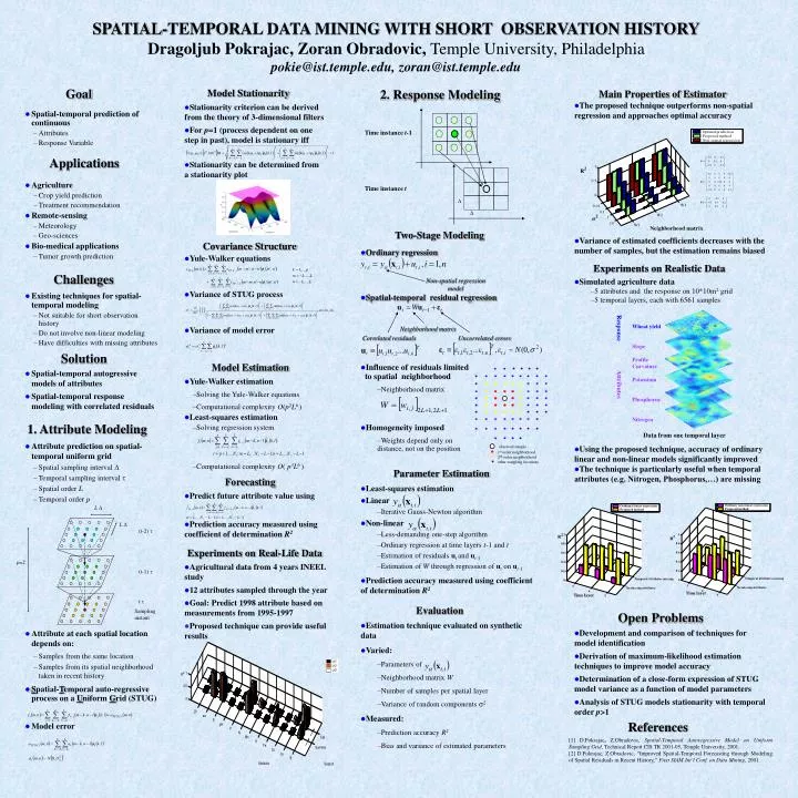
1. Time instance t-1 Response Wheat yield Slope Profile Curvature Potassium Phosphorus Nitrogen Time instance t Attributes observed sample  1st order neighborhood 2nd order neighborhood  other sampling locations 2 2 1 1 p p L L (t-2)  p=2 (t-1)  t  Sampling instant SPATIAL-TEMPORAL DATA MINING WITH SHORT OBSERVATION HISTORYDragoljub Pokrajac,Zoran Obradovic,Temple University, Philadelphiapokie@ist.temple.edu, zoran@ist.temple.edu Goal 2. Response Modeling • Model Stationarity • Stationarity criterion can be derived from the theory of 3-dimensional filters • For p=1 (process dependent on one step in past), model is stationary iff • Stationarity can be determined from a stationarity plot • Yule-Walker equations • Variance of STUG process • Variance of model error • Yule-Walker estimation • Solving the Yule-Walker equations • Computational complexity O(p2L6 ) • Least-squares estimation • Solving regression system • Computational complexity O( p3L6 ) • Predict future attribute value using • Prediction accuracy measured using coefficient of determination R2 • Agricultural data from 4 years INEEL study • 12 attributes sampled through the year • Goal: Predict 1998 attribute based on measurements from 1995-1997 • Proposed technique can provide useful results Main Properties of Estimator • The proposed technique outperforms non-spatial regression and approaches optimal accuracy • Variance of estimated coefficients decreases with the number of samples, but the estimation remains biased • Simulated agriculture data • 5 attributes and the response on 10*10m2 grid • 5 temporal layers, each with 6561 samples • Using the proposed technique, accuracy of ordinary linear and non-linear models significantly improved • The technique is particularly useful when temporal attributes (e.g. Nitrogen, Phosphorus,…) are missing • Development and comparison of techniques for model identification • Derivation of maximum-likelihood estimation techniques to improve model accuracy • Determination of a close-form expression of STUG model variance as a function of model parameters • Analysis of STUG models stationarity with temporal order p>1 • Spatial-temporal prediction of continuous • Attributes • Response Variable • Agriculture • Crop yield prediction • Treatment recommendation • Remote-sensing • Meteorology • Geo-sciences • Bio-medical applications • Tumor growth prediction • Existing techniques for spatial-temporal modeling • Not suitable for short observation history • Do not involve non-linear modeling • Have difficulties with missing attributes • Spatial-temporal autogressive models of attributes • Spatial-temporal response modeling with correlated residuals • Attribute prediction on spatial-temporal uniform grid • Spatial sampling interval  • Temporal sampling interval  • Spatial order L • Temporal order p • Attribute at each spatial location depends on: • Samples from the same location • Samples from its spatial neighborhood taken in recent history • Spatial-Temporal auto-regressive process on a Uniform Grid (STUG) • Model error Applications Two-Stage Modeling Covariance Structure • Ordinary regression • Spatial-temporal residual regression • Influence of residuals limited to spatial neighborhood • Neighborhood matrix • Homogeneity imposed • Weights depend only on distance, not on the position • Least-squares estimation • Linear • Iterative Gauss-Newton algorithm • Non-linear • Less-demanding one-step algorithm • Ordinary regression at time layers t-1 and t • Estimation of residuals ut and ut-1 • Estimation of W through regression of ut on ut-1 • Prediction accuracy measured using coefficient of determination R2 • Estimation technique evaluated on synthetic data • Varied: • Parameters of • Neighborhood matrix W • Number of samples per spatial layer • Variance of random components 2 • Measured: • Prediction accuracy R2 • Bias and variance of estimated parameters Experiments on Realistic Data Challenges Non-spatial regression model Neighborhood matrix Correlated residuals Uncorrelated errors Solution Model Estimation 1. Attribute Modeling Data from one temporal layer Parameter Estimation Forecasting Experiments on Real-Life Data Evaluation Open Problems References [1] D.Pokrajac, Z.Obradovic, Spatial-Temporal Autoregressive Model on Uniform Sampling Grid, Technical Report CIS TR 2001-05, Temple University, 2001. [2] D.Pokrajac, Z.Obradovic, “Improved Spatial-Temporal Forecasting through Modeling of Spatial Residuals in Recent History,” First SIAM Int’l Conf. on Data Mining, 2001.