Download
1 / 32
320 likes | 439 Views
Non-Stationarity in the circulation-climate relationship Stability of NAO-Influence on the Regional Climate of the Baltic Sea Area Possible Effects on NAO-Reconstructions?. (1) Frederik Schenk, Sebastian Wagner, Eduardo Zorita (2) Daniel Hansson.

E N D
Non-Stationarity in the circulation-climate relationship Stability of NAO-Influence on the Regional Climate of the Baltic Sea Area Possible Effects on NAO-Reconstructions? (1) Frederik Schenk, Sebastian Wagner, Eduardo Zorita (2) Daniel Hansson (1) GKSS Research Center Geesthacht – Institute for Coastal Research – System Analysis and Modeling (2) Göteborg University – Earth Sciences Center – Ocean Climate Group
Outline • 1 Non-Stationarity in Observations • - spatiotemporal changes of NAO-control on regional climate • 2 Non-Stationarity in Climate Model Simulations • - temporal evolution of the NAO-t2m-relationship over 990 years • 3 Idealized pseudo-proxy reconstruction of NAO from local-scale • 4 Summary
Assumption of Stationarity in Climate Reconstructions • Most statistical reconstructions assume stationarity between climate circulation and regional climate impact (proxy location) • i.e. linear relationship between NAO and near-surface climate Local climate = F(large-scale + x) physical assumption: Residuum not captured by linear equation Regional climate or local proxy Proportional constant Large scale i.g. PC
First leading EOFs of 1000-1990 PCA calculates covariability matrix of SLP field anomalies
1 Non-Stationarity in observations The NAO – temperature relationship
http://www.baltex-research.eu/BACC/media/ Definition of circulation indices and T-Baltic from Echo-G and Luterbacher-SLP-reconstruction
Detection of Non-Stationarity • Non-Stationarity • =: changes in strength of a relationship between two climate variables • - expressed as Running Correlation coefficients over time (Pearson) • - window size of 31 years = RC30
Data • Surface Temperature (t2m) • Long historical station temperatures • T-Baltic (t2m) of different AOGCM simulations from ECHO-G • MIB (Max. sea-Ice extent of the Baltic Sea) • MIB (obs.) (Seinä & Palosuo 1996) • MIB (mod.) – box-model PROBE-Baltic (Hansson & Omstedt 2007) • Circulation indices • NAO of Azores minus Iceland (Jones et al. 1997) • NAO from 500 year SLP-reconstruction (Luterbacher et al. 2002) • NAO from SLP of different simulations from ECHO-G • with different forcings and initial conditions
NAO and sea-ice (MIB) Hansson, D. & A. Omstedt (2007): Modelling the Baltic Sea ocean climate on centennial time scale: temperature and sea ice. Climate Dynamics 30, 763-778
2 Non-Stationarity in Climate Model Simulations 990 year model study from AOGCM Echo-G
Climate Model Simulations • Climate simulation as a surrogate climate: • - Model = simplified representation of „real“ processes • Idealized pseudo-reconstruction-approach: • - comparison of NAO and CEZI • - use of area weighted t2m of the Baltic catchment area for • reconstructing the NAO by simple linear regression (without • adding white noise) • - comparison with „real“ model NAO • - estimation of non-stationarity for reconstructions within the model
Atmosphere: ECHAM4 T30 (3.75° x 3.75°) 19 vertical layers Ocean: HOPE-G Horizontal Resolution 2,81° x 2,81° 20 vertical layers increased tropical resolution Model description of Echo-G
Settings of Echo-G simulations • Control-run of 1000 model years with fixed present conditions • External forced simulations I: solar + volcanic + greenhouse Gases • ERIK1: 990-1990 A.D. starting with warm ocean as initial condition • ERIK2: 990-1990 A.D. starting with cold ocean as initial condition • External forced simulations II: + orbital forcing • Oetzi1: 7000 B.P. – 1998 A.D. with orbital forcing only • Oetzi2: 7000 B.P. – 1998 A.D. with orbital, solar and greenhouse gases (no volcanic)
NAO vs. Baltic Sea climateexternal forced (solar, volcanic, GHG)
3 Idealized pseudo-proxy reconstruction of NAO from local scale
Idealized pseudo-reconstruction estimation of NAO from pseudo-proxy
4 Summary • Magnitude of non-stationarity for NAO-impact is high for Baltic Sea area • - NAO vs. station-temperature 1824-2008 (DJF): RC30 = {10 - 65%} • - NAO vs. sea-ice (MIB) since 1500: RC30 = {0 – 64%} • - NAO vs. t2m (AOGCM) (DJF) since 1000: RC30 = {0 – 64%}
4 Summary • Comparison of external forced simulations with control-run (990 years): • - same magnitude of non-stationarity over time with all/no forcings • - no relationship between forcing and non-stationarity • non-stationarity is mainly result of internal climate variability • possible external influence on longer time scales (orbital changes)? • e.g. Groll et al. (2005):Changes in AO-regional-climate relationship during Eemian (125 kyr BP) compared with pre-industrial (1800 A.D.) • - significantly lower AO-t2m signal for NH winter during Eemian • - also stronger NH winter westerlies towards Europe, warmer CET Groll, N., Widmann, M., Jones, J., Kaspar, F. & S. Lorenz (2005): Simulated relationship between regional temperatures and large-scale circulation: 125 kyr BP (Eemain) and the preindustrial period Journal of Climate 2005, 18(19), 4032-4045
References • Cassou, C., L. Terray, J.W. Hurrell and C. Deser (2004): North Atlantic winter climate regimes: spatial asymmetry, stationarity with time and oceanic forcing, J. Climate, 17, 1055-1068. • Hansson, D. & A. Omstedt (2007): Modelling the Baltic Sea ocean climate on centennial time scale: temperature and sea ice. Climate Dynamics 30, 763-778 • Jacobeit, J., Beck, C. & A. Philipp (1998): Annual to Decadal Variability in Climate in Europe. Würzburger Geographische Mauskripte, Vol. 43. • Luterbacher, J., Xoplaki, E., Dietrich, D., Rickli, R., Jacobeit, J., Beck, C., Gyalistris, D., Schmutz, C. & H. Wanner (2002): Reconstruction of sea level pressure fields over Eastern North Atlantic and Europe back to 1500. Clim. Dyn. 18: 545-561. • Osborn, T.J., Briffa, K.R., Tett, S.F.B., Jones, P.D. and R.M. Trigo (1999): Evaluation of the North Atlantic Oscillation as simulated by a coupled climate model. Climate Dynamics 15, 685-702. • Vicente-Serrano, S. M., and J. I. López-Moreno (2008), Nonstationary influence of the North Atlantic Oscillation on European precipitation, J. Geophys. Res., 113. • Zorita, E. and F. González-Rouco (2002): Are temperature-sensitive proxies adequate for North Atlantic Oscillation reconstructions? Geophysical Research Letters, 29 (14), 48-1 - 48-4. • Zorita, E., Gonzalez-Rouco, F. and S. Wagner (2009): Low-frequency response of the Arctic Oscillation to external forcing in the past millennium. Geophysical Research Letters (submitted).
Thank you for your attention! Climate is what we expect, Weather is what we get. (after Lorenz)
5 Outlook Principal Component Analysis teleconnection patterns describe the low-frequency extratropical atmosphere generally in terms of space-stationary and time-fluctuating structures
Stability of SLP-patterns over time:Running EOF • Moving-EOF-analysis with window size a = 31years • Comparison of reference patterns (EOFs over 1000-1998) with subperiods • Field-correlation detected by |scalarproduct| of reference pattern R of the whole time period with each subperiod-EOF S yields |rR,S| = [0,1] • with • |r| = [0,1] due to orthogonality of EOFs • * Field correlations like RunCor(X,Y) of anomaly field with mean
__Changes of westerly winds in the North Atlantic region _Temporal evolution of the DJF North Atlantic Oscillation Index Zorita, E., Gonzalez-Rouco, F. and S. Wagner (2009): Low-frequency response of the Arctic Oscillation to external forcing in the past millennium. Geophysical Research Letters (submitted).