Download
1 / 16
160 likes | 510 Views
Interpretability vs. out-of-sample prediction performance in spatial hedonic models. Bjarke Christensen, Sydbank Tony Vittrup Sørensen, Jyske Bank. Outline. Spatial autocorrelation in hedonic house price models The data Related literature Methods Results Concluding remarks. Motivation.

E N D
Interpretability vs. out-of-sample prediction performance in spatial hedonic models Bjarke Christensen, Sydbank Tony Vittrup Sørensen, Jyske Bank
Outline • Spatial autocorrelation in hedonic house price models • The data • Related literature • Methods • Results • Concluding remarks
Motivation • Two uses for hedonic house price models: • Forecasting future sales prices (AVM, mass appraisal). • Estimating implicit value of externalities/amenities • Spatial autocorrelation: a curse, and a blessing? • Causes biased and inconsistent parameter estimates • Can be used to improve forecast precision • Methods for ‘dealing with’ spatial autocorrelation include • Fixed effects / GIS variables • Spatial econometric models • Semiparametric / spline based models an alternative? (von Grewnitz and Panduro (LE, 2014)).
Motivation • Does the objective dictate the approach? • For forecasting, interpretability is desirable but less important than accuracy • For externalities, interpretability is paramount • The spatial variable of interest in this presentation is: proximity to wind turbines.
Data • Western Jutland, 8 municipalities, 7.000 km2. • Period: 2002-2014 • Number of single family property sales: • In-sample: 21.066 • Out-of-sample: 2.340 • Control variables: living area, number of rooms, age, number of bathrooms, detached vs. semi-detached, roof material, exterior wall material, proximity to large road.
Spatial variable of interest: wind turbines • Provided 30% of electric power consumption in Denmark in 2012. • Expected to increase to 50% in 2020. • Neighbours legally entitled to compensation for ‘loss of property value’.
Methods • Ordinary least squares • Spatial Error Model • Anselin. (1988). • Generalized additive model • Wood et al. (JRSS, 2008). • Interpretability
Estimation strategies • Hedonic models with a small set of controls, varying only the spatial approach • The proximity of a windmill is estimated as 1.5 km less the distance to the nearest active windmill • The OLS model serves as a baseline • SEM models • Row-standardized, k-nearest neighbours spatial weight matrix • Number of neighbours ranges from 5 to 50 • Fitting by Maximum Likelihood • GAM models • Maximum number of knots ranges from 50 to 2000 • Penalized least squares, penalty determined by generalized cross validation • Compare estimates to • Out-of-sample prediction errors • Median absolute percentage error • Tests for spatial autocorrelation • Moran’s I, Perturbed Moran’s I, Geary’s C, Perturbed Geary’s C
Additional results - GAM models Knots Resid. Df Resid. Dev Df Deviance F Pr(>F) 50 20948 1566.9 250 20768 1227.5 179.99 339.43 36.7015 < 2.2e-16 *** 500 20594 1165.2 174.41 62.24 6.9450 < 2.2e-16 *** 750 20387 1118.1 206.43 47.11 4.4412 < 2.2e-16 *** 1000 20215 1085.3 172.22 32.85 3.7118 < 2.2e-16 *** 1500 20089 1051.8 126.27 33.42 5.1510 < 2.2e-16 *** 2000 19956 1025.4 132.50 26.45 3.8850 < 2.2e-16 *** --- Signif. codes: 0 ‘***’ 0.001 ‘**’ 0.01 ‘*’ 0.05 ‘.’ 0.1 ‘ ’ 1
Additional results - Spatial autocorrelation tests
Where did the externality go? • Omitted variable bias / inconsistent estimates? • Concurvity between distance measure and the spatial modelling?
The soap-film surface: model comparison k=50 k=2000