Download

1 / 26
260 likes | 273 Views
Explore the evolution of logic synthesis from Verilog to gate arrays, standard cells, and silicon compilers. Understand the tools, optimizations, and shift in design emphasis over the years. Learn about synthesis processes, HDL semantics, simulation, and the inference of logic elements.

E N D
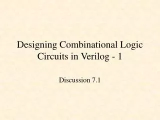
A Instruction A B Memory D mux 1 0 Synthesis: Verilog Gates // 2:1 multiplexer always @(sel or a or b) begin if (sel) z <= b; else z <= a; end Gate Library
Some History ... In late 70’sMead-Covway showed how to lay out transistors systematically to build logic circuits. Tools: Layout editors, for manual design; Design rule checkers, to check for legal layout configurations; Transistor-level simulators; Software generators to create dense transistor layouts; 1980 : Circuits had 100K transistors In80’sdesigners moved to the use of gate arrays and standardized cells, pre-characterized modules of circuits, to increase productivity. Tools: To automatically place and route a netlist of cells from a predefined cell library The emphasis in design shifted to gate-level schematic entry and simulation
History continued... By late 80’s designers found it very tedious to move a gate-level design from one library to another because libraries could be very different and each required its own optimizations. Tools: Logic Synthesis tools to go from Gate netlists to a standard cell netlist for a given cell library. Powerful optimizations! Simulation tools for gate netlists, RTL; Design and tools for testability, equivalance checking, ... IBM and other companies had internal tools that emphasized top down design methodology based on logic synthesis. Two groups of designers came together in 90’s: Those who wanted to quickly simulate their designs expressed in some HDL and those who wanted to map a gate-level design in a variety of standard cell libraries in an optimized manner.
a.k.a. “silicon compilers” Synthesis Tools Idea: once a behavioral model has been finished why not use it to automaticallysynthesizea logic implementation in much the same way as a compiler generates executable code from a source program? Synthesis programs process the HDL then 1 infer logic and state elements 2 perform technology-independent optimizations (e.g., logic simplification, state assignment) 3 map elements to the target technology 4 perform technology-dependent optimizations (e.g., multi-level logic optimization, choose gate strengths to achieve speed goals)
Simulation vs Synthesis In a HDL like Verilog or VHDL not every thing that can be simulated can be synthesized. There is a difference between simulation and synthesis semantics. Simulation semantics are based on sequential execution of the program with some notion of concurrent synchronous processes. Not all such programs can be synthesized. It is not easy to specify the synthesizable subset of an HDL So in today’s lecture we will gloss over 1, briefly discuss 2 and emphasize 3 and 4. 1 infer logic and state elements 2 perform technology-independent optimizations (e.g., logic simplification, state assignment) 3 map elements to the target technology 4 perform technology-dependent optimizations (e.g., multi-level logic optimization, choose gate strengths to achieve speed goals)
Logic Synthesis a b z assign z = (a & b) | c; c a b z c a // dataflow assign z = sel ? a : b; 1 z 0 b sel a sel z b
sum[0] sum[2] sum[1] sum[3] fulladder fulladder fulladder fulladder cout 0 x[0] y[0] x[1] y[1] x[2] y[2] x[3] y[3] Logic Synthesis (II) wire [3:0] x,y,sum; wire cout; assign {cout,sum} = x + y; As a default + is implemented as a ripple carry editor
Logic Synthesis (III) module parity(in,p); parameter WIDTH = 2; // default width is 2 input [WIDTH-1 : 0] in; output p; // simple approach: assign p = ^in; // here's another, more general approach reg p; always @(in) begin: loop integer i; reg parity = 0; for (i = 0; i < WIDTH; i = i + 1) parity = parity ^ in[i]; p <= parity; end endmodule … wire [3:0] word; wire parity; parity #(4) ecc(word,parity); // specify WIDTH = 4 word[3] parity word[2] word[1] word[0] XOR with “0” input has been optimized away…
Synthesis of Sequential Logic reg q; // D-latch always @(g or d) begin if (g) q <= d; end d q D Q G g If q were simply a combinational function of d, the synthesizer could just create the appropriate combinational logic. But since there are times when the always block executes but q isn’t assigned (e.g., when g = 0), the synthesizer has to arrange to remember the value of “old” value q even if d is changing it will infer the need for a storage element (latch, register, …). Sometimes this inference happens even when you don’t mean it to – you have to be careful to always ensure an assignment happens each time through the block if you don’t want storage elements to appear in your design. reg q; // this time we mean it! // D-register always @(posedge clk) begin q <= d; end d q D Q clk
Sequential Logic (II) reg q; // register with synchronous clear always @(posedge clk) begin if (!reset) // reset is active low q <= 0; else q <= d; end d q D Q reset clk reg q; // register with asynchronous clear always @(posedge clk or negedge reset) begin if (!reset) // reset is active low q <= 0; else// implicit posedge clk q <= d; end // warning! async inputs are dangerous! // there’s a race between them and the // rising edge of clk. d q D Q clk reset
Technology-independent* optimizations • Two-level boolean minimization: based on the assumption that reducing the number of product terms in an equation and reducing the size of each product term will result in a smaller/faster implementation. • Optimizing finite state machines: look for equivalent FSMs (i.e., FSMs that produce the same outputs given the same sequence of inputs) that have fewer states. • Choosing FSM state encodings that minimize implementation area (= size of state storage + size of logic to implement next state and output functions). * None of these operations is completely isolated from the target technology. But experience has shown that it’s advantageous to reduce the size of the problem as much as possible before starting the technology-dependent optimizations. In some places (e.g. the ratio of the size of storage elements to the size logic gates) our assumptions will be valid for several generations of the technology.
Two-Level Boolean Minimization • Two-level representation for a multiple-output Boolean function: • - Sum-of-products • Optimization criteria: • - number of product terms • - number of literals • - a combination of both • Minimization steps for a given function: • Generate the set of prime product-terms for the function • Select a minimum set of prime terms to cover the function. • State-of-the-art logic minimization algorithms are all based onthe Quine-McCluskey method and follow the above two steps.
Prime Term Generation W X Y Z label 0 0 0 0 0 0 1 0 1 5 0 1 1 1 7 1 0 0 0 8 1 0 0 1 9 1 0 1 0 10 1 0 1 1 11 1 1 1 0 14 1 1 1 1 15 Express your Boolean function using 0-terms (product terms with no don’t care care entries). Include only those entries where the output of the function is 1 (label each entry with it’s decimal equivalent). 0-terms: Look for pairs of 0-terms that differ in only one bit position and merge them in a 1-term (i.e., a term that has exactly one ‘–’ entry). 0, 8 -000 5, 7 01-1 7,15 -111 8, 9 100- 8,10 10-0 9,11 10-1 10,11 101- 10,14 1-10 11,15 1-11 14,15 111- [A] [B] [C] 1-terms: Next 1-terms are examined in pairs to see if the can be merged into 2-terms, etc. Mark k-terms that get merged into (k+1) terms so we can discard them later. 2-terms: [D] [E] 8, 9,10,11 10-- 10,11,14,15 1-1- Label unmerged terms: these terms are prime! Example due to Srini Devadas 3-terms: none!
Prime Term Table An “X” in the prime term table in row R and column C signifies that the 0-term corresponding to row R is contained by the prime corresponding to column C. A B C D E 0000 X . . . . 0101 . X . . . 0111 . X X . . 1000 X . . X . 1001 . . . X . 1010 . . . X X 1011 . . . X X 1110 . . . . X 1111 . . X . X Goal: select the minimum set of primes (columns) such that there is at least one “X” in every row. This is the classical minimum covering problem. A is essential B is essential D is essential E is essential Each row with a single X signifies an essential prime term since any prime implementation will have to include that prime term because the corresponding 0-term is not contained in any other prime. In this example the essential primes “cover” all the 0-terms.
Dominated Columns Some functions may not have essential primes (Fig. 1), so make arbitrary selection of first prime in cover, say A (Fig. 2). A column U of a prime term table dominates V if U contains every row contained in V. Delete the dominated columns (Fig. 3). 1. Prime table 2. Table with A selected 3. Table with B & H removed A B C D E F G H B C D E F G H C D E F G0000 X . . . . . . X 0101 X X . . . . . 0101 X . . . .0001 X X . . . . . . 0111 . X X . . . . 0111 X X . . .0101 . X X . . . . . 1000 . . . . . X X 1000 . . . . X0111 . . X X . . . . 1010 . . . . X X . 1010 . . . X X1000 . . . . . . X X 1110 . . . X X . . 1110 . . X X .1010 . . . . . X X . 1111 . . X X . . . 1111 . X X . .1110 . . . . X X . .1111 . . . X X . . . C is essential G is essential C dominates B, G dominates H Selecting C and G shows that only E is needed to complete the cover This gives a prime cover of {A, C, E, G}. Now backtrack to our choice of A and explore a different (arbitrary) first choice; repeat, remembering minimum cover found during search.
The Quine-McCluskey Method The input to the procedure is the prime term table T. 1. Delete the dominated primes (columns) in T. Detect essential primes in T by checking to see if any 0-term is contained by a single prime. Add these essential primes to the selected set. Repeat until no new essential primes are detected. 2. If the size of the selected set of primes equals or exceeds the best solution thus far return from this level of recursion. If there are no elements left to be contained, declare the selected set as the best solution recorded thus far. 3. Heuristically select a prime. 4. Add the chosen prime to the selected set and create a new table by deleting the prime and all 0-terms that are contained by this prime in the original table. Set T to this new table and go to Step 1.Then, create a new table by deleting the chosen prime from the original table without adding it to the selected set. No 0-terms are deleted from the original table. Set T to new table and go to Step 1. The good news: this technique generalizes to multi-output functions (see the QM handout on the website for details). The bad news: the search time grows as 2^(2^N) where N is the number of inputs. So most modern minimization systems use heuristics to make dramatic reductions in the processing time.
Mapping to target technology • Once we’ve minimized the logic equations, the next step is mapping each equation to the gates in our target gate library. • Popular approach: DAG covering (K. Keutzer)
Mapping Example Problem statement: find an “optimal” mapping of this circuit: Into this library: Example due to Kurt Keutzer
2-input NAND gates + inverters DAG Covering • Represent input netlist in normal form (“subject DAG”). • Represent each library gate in normal form (“primitive DAGs”). • Goal: find a minimum cost covering of the subject DAG by the primitive DAGs. • If the subject and primitive DAGs are trees, there is an efficient algorithm (dynamic programming) for finding the optimum cover. • So: partition subject DAG into a forest of trees (each gate with fanout > 1 becomes root of a new tree), generate optimal solutions for each tree, stitch solutions together.
Primitive DAGs for library gates 8 13 13 10 11
Possible Covers Hmmm. Seems promising but is there a systematic and efficient way to arrive at the optimal answer?
Use dynamic programming! Principle of optimality: Optimal cover for a tree consists of a best match at the root of the tree plus the optimal cover for the sub-trees starting at each input of the match. Best cover for this match uses best covers for P, X & Y X Z Y Complexity: To determine the optimal cover for a tree we only need to consider a best-cost match at the root of the tree (constant time in the number of matched cells), plus the optimal cover for the subtrees starting at each input to the match (constant time in the fanin of each match) O(N) P Best cover for this match uses best covers for P & Z
Example (III) Yes Regis, this is our final answer. This matches our earlier intuitive cover, but accomplished systematically. Refinements: timing optimization incorporating load-dependent delays, optimization for low power.
Technology-dependent optimizations • Additional library components: more complex cells may be slower but will reduce area for logic off the critical path. • Load buffering: adding buffers/inverters to improve load-induced delays along the critical path • Resizing: Resize transistors in gates along critical path • Retiming: change placement of latches/registers to minimize overall cycle time • Increase routability over/through cells: reduce routing congestion. You are here! Gate netlist Logic Synthesis Place & route Verilog Mask • HDL logic • map to target library • optimize speed, area • create floorplan blocks • place cells in block • route interconnect • optimize (iterate!)