Relative Velocity, Velocity Gradient, and Deformation Shear Deformation

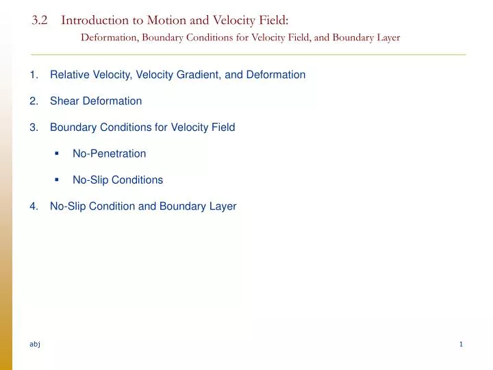
1. 3.2 Introduction to Motion and Velocity Field: Deformation, Boundary Conditions for Velocity Field, and Boundary Layer • Relative Velocity, Velocity Gradient, and Deformation • Shear Deformation • Boundary Conditions for Velocity Field • No-Penetration • No-Slip Conditions • No-Slip Condition and Boundary Layer

2. Very Brief Summary of Important Points and Equations • Deformation In order to have deformation, • relative velocity between neighboring point , or • velocity (spatial) gradient is required. • Boundary condition for velocity field at a solid wall • Boundary Layer: Thin shear layer near a solid wall where [because of no-slip condition (and viscous effect)] shear stress is relatively large and viscous/frictional effect is important.

3. B B t A B t + dt t t + dt A B A A Relative velocity in the transverse direction: Relative velocity in the axial direction: B B t A B t t + dt t + dt A B A A If , no deformation. If , no deformation. If , shear deformation (/rotation –component of). If , deformation/stretching. Relative Velocity, Velocity Gradient, and Deformation (Rate) • In other words, in order to have deformation, • relative velocity between neighboring point , or • velocity (spatial) gradient is required.

4. d l d u = uB – uA= relative velocity of B with respect to A B (t) B (t + d t) Fluid element at time t + d t d y d a Fluid element at time t A Shear deformation rate = Dimension: Shear deformation rate = Shear Deformation Rate / Shear Strain Rate

5. y Smaller du/dy at B – lower shear deformation rate Velocity profile at x = xo B Larger du/dy at A– higher shear deformation rate A x u x = xo Velocity Profile (and Shear Deformation Rate) • u = u (y): The plot of the variation of the velocity u with the transverse coordinate y is referred to as the velocity profile.

6. From The Japan Society of Mechanical Engineers, 1988, Visualized flow: Fluid motion in basic and engineering situations revealed by flow visualization, Pergamon Press. Flow Image

7. w Fluid Boundary Conditions: No-Penetration / No-Slip Conditions • Consider the relative velocity of fluid with respect to a solid wall: • Let = fluid velocity wrt earth at point w on the wall • = solid wall velocity wrt earth at point w on the wall • Hence, the relative velocity of fluid wrt the solid wall at w is given by • Decomposing the relative velocity into the normal (to the local surface) and tangential components:

8. Real: No-slip / No-penetration Ideal: Free-slip / No-penetration w • Hence, (for impermeable wall) • for real fluid/flow • for ideal fluid/flow • For an impermeable wall, fluid cannot penetrate into solid, hence the normal component of the relative velocity vanishes. • This is called no-penetration condition. • This is not the case for, e.g., porous wall. For ideal fluid/flow: free-slip (No constraint) For real fluid/flow, it is observedno-slip

9. Freestream: Low du/dy  Lowtyx approximately inviscid region. Freestream velocity Viscous/frictional stress Flow Boundary Layer: high du/dy hightyx highly viscous region. Solid wall Zero fluid velocity at the wall (no slip) No-Slip Condition, Viscosity, and Boundary Layer Laminar boundary layer (From Van Dyke, M., 1982, An Album of Fluid Motion, Parabolic Press.) • Due to no-slip condition at the solid wall, fluid velocity decreases from the value in the freestream to zero value at the wall as the wall is approached. • This creates a thin layer of highdu/dy, and thus a highly viscous region. This thin region is called boundary layer.

10. Freestream velocity Solid wall No-slip Decreasing velocity as the wall is approached. Outside flow is ~ inviscid Boundary layer is highly viscous

11. y y Still air B B Flow U x A A Plate is moving at the speedU. Flow between two stationary parallel plates (Channel flow) Example: Qualitatively sketch velocity profile from the knowledge of BC • Use the knowledge of the boundary condition for a velocity field to qualitatively sketch the velocity profile along the traverse AB • Assume that the only dominant velocity isu (Vx)