Download
1 / 29
300 likes | 538 Views
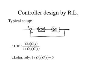
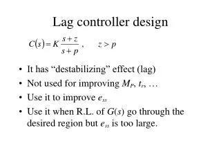
Controller design by R.L. Typical setup:. C(s). G(s). Controller Design Goal: Select poles and zero of C(s) so that R.L. pass through desired region Select K corresponding to a good choice of dominant pole pair. Types of classical controllers. Proportional control

E N D
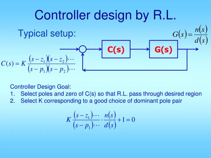
Controller design by R.L. Typical setup: C(s) G(s) Controller Design Goal: Select poles and zero of C(s) so that R.L. pass through desired region Select K corresponding to a good choice of dominant pole pair
Types of classical controllers • Proportional control • Needed to make a specific point on RL to be closed-loop system dominant pole • Proportional plus derivative control (PD control) • Needed to “bend” R.L. into the desired region • Lead control • Similar to PD, but without the high frequency noise problem; max angle contribution limited to < 75 deg • Proportional plus Integral Control (PI control) • Needed to “eliminate” a non-zero steady state tracking error • Lag control • Needed to reduce a non-zero steady state error, no type increase • PID control • When both PD and PI are needed, PID = PD * PI • Lead-Lag control • When both lead and lag are needed, lead-lag = lead * lag
Proportional control design • Draw R.L. for given plant • Draw desired region for poles from specs • Pick a point on R.L. and in desired region • Use ginput to get point and convert to complex # • Compute • Obtain closed-loop TF • Obtain step response and compute specs • Decide if modification is needed nump=…; denp= …; sysp=tf(nump, denp); rlocus(sysp); [x,y]=ginput(1); pd=x+j*y; Gpd=evalfr(sysp,pd); K=1/abs(Gpd); sysc = K; syscl = feedback(sysc*sysp,1); use your program from several weeks ago to do all these
Example code for Matlab rlocus([9], [1 8 12 0]); grid; yl=ylim; omega_n=5; %this may be from tr or td requirement rectangle('Position',[-omega_n,-omega_n,2*omega_n,2*omega_n],'Curvature',[1,1]); sigma = 4; %this may be from ts requirement line([-sigma -sigma],yl); zeta=0.7; %this may be from Mp requiremet line([0 yl(1)*zeta/sqrt(1-zeta^2)],[0 yl(1)]); line([0 -yl(2)*zeta/sqrt(1-zeta^2)],[0 yl(2)]); xl=xlim; xl(2)=0; xlim(xl); Draws circle with r=5 Draws line at -4 Draws 2 rays for zeta=0.7
PD controller design • This is introducing an additional zero to the R.L. for G(s) • Use this if the dominant pole pair branches of G(s) do not pass through the desired region • Place additional zero to “bend” the RL into the desired region
Design steps: • From specs, draw desired region for pole.Pick from region, not on RL • Compute • Select • Select: [x,y]=ginput(1); pd=x+j*y; Gpd=evalfr(sys_p,pd) phi=pi - angle(Gpd) z=abs(real(pd))+abs(imag(pd)/tan(pi-phi)) Kd=1/abs(pd+z)/abs(Gpd)
C(s) Example: Want: Sol: (pd not on R.L.) (Need a zero to attract R.L. to pd)
ts is OK But Mp too large To redesign: Reduce wd pd=-2+j1.5
Gpd = evalfr(sys_p, pd) Gpd = - 0.1600 + 0.2133i phi = pi - angle(Gpd) phi = 0.9273 z = abs(real(pd)) + abs(imag(pd)/tan(pi - phi)) z = 3.1250 Kd = 1/abs(pd+z)/abs(Gpd) Kd = 2 Kp = z*Kd Kp = 6.2500 sys_c=tf([Kd Kp], 1); sys_cl=feedback(sys_c*sys_p, 1) Transfer function: 2 s + 6.25 ---------------- s^2 + 4 s + 6.25 step(sys_cl); ylim([0 yss*(1+2*Mp)])
Drawbacks of PD • Not proper : deg of num > deg of den • High frequency gain → ∞: • High gain for noise Saturates circuits Cannot be implemented physically
Lead Controller • Approximation to PD • Same usefulness as PD • It contributes a lead angle:
Approximation to PD • Same usefulness as PD • Lead Control: • Draw R.L. for G • From specs draw region for desired c.l. poles • Select pd from region • LetPick –z somewhere below pd on –Re axisLetSelect [x,y]=ginput(1); pd=x+j*y; Gpd=evalfr(sysp,pd) phi=pi - angle(Gpd) [x,y]=ginput(1); z=abs(x); phi1=angle(pd+z); phi2=phi1-phi; p=abs(real(pd))+abs(imag(pd)/tan(phi2)); K=abs((pd+p)/(pd+z)/Gpd); sysc=tf(K*[1 z],[1 p]); Hold on; rlocus(sysc*sysp);
Example: Lead Design MP is fine, but too slow. Want: Don’t increase MP but double the resp. speed Sol: Original system: C(s) = 1 Since MP is a function of ζ, speed is proportional to ωn C(s)
Draw R.L. & desiredregion Pick pd right at the vertex: (Could pick pd a little inside the region to allow “flex”)
Clearly, R.L. does not pass through pd, nor the desired region.need PD or Lead to “bend” the R.L. into region.(Note our choice may be the easiest to achieve) Let’s do Lead:
Change controller from to To reduce the gain a bit, and make it a little closer to PD
Lead Control with angle bisector • Draw R.L. for G • From specs draw region for desired c.l. poles • Select pd from region • Let • Select phipd=angle(pd); phi1=(phipd+phi)/2; phi2=phi1-phi;