Download
1 / 30
300 likes | 452 Views
Introduction to Atmospheric Climate Modeling (CAM within CCSM) Phil Rasch. What is CCSM?. Strat Chem WACCM. Aerosols. Atmosphere (CAM3). Isotopes (H,C,O ). Trop Chem Aerosols. Bio Geochemistry. Ocean (POP). Coupler (CPL6). Sea Ice (CSIM5). Isotopes (H,C,O ). Land (CLM3).

E N D
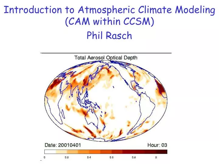
Introduction to Atmospheric Climate Modeling(CAM within CCSM)Phil Rasch
What is CCSM? Strat Chem WACCM Aerosols Atmosphere(CAM3) Isotopes (H,C,O) Trop Chem Aerosols BioGeochemistry Ocean (POP) Coupler (CPL6) Sea Ice (CSIM5) Isotopes (H,C,O) Land (CLM3) Isotopes (H,C,O) BioGeochemistry Dynamic Vegetation
Some comments on CCSM configurations • All components can be interactive • All components can be replaced with “data models” • Information about that component is prescribed --- read in from an external dataset • CAM can be run with • Full interaction • As a Chemical Transport Model(acts as a processor and conduit for exchangebetween other model components)
Implementation Details in the atmosphere of possibleinterest to the class • Model performs sequential applications of a number of physical processes • State variables (temperature, winds, density, water substances, trace constituents) are updated after each process representation is applied • We typically divide processes into two classes • “Dynamics” (the equations of motion = Navier Stokes equations simplified to assume hydrostatic balance in the vertical) • Dynamics = dynamical core = instantaneous solution requires information in latitude, longitude, and height! • “Physics” (diabatic processes such as radiative transfer, processes involving water phase change, chemistry, etc) • Physics = parameterizations = solutions generally only require information in height = work on a column by column basis • “Transport” (sometimes)
Time Loop Dynamics Dry Adiabatic LapseRate Adjustment Chemistry Moist DeepConvection Shallow Convection Boundary Layer Processes Stratiform Clouds, Wet Chemistry, Aerosols Coupling to land/ocean/ice Radiation
CAM dynamical configurations available for use • Spectral dynamics, semi-Lagrangian transport (SLT) for tracers --- Traditional • Spherical harmonic discretization in horizontal • Low order finite differences in vertical • Inconsistent, Non-conservative -> fixers required for tracers • Semi-Lagrangian Dynamics, semi-Lagrangian Transport for tracers • Polynomial representation of evolution of “mixing ratios” for all fields • Inconsistent, Non-conservative -> fixers required for tracers • Finite Volume (FV) using “flux form semi-Lagrangian” framework of Lin and Rood • Semi-consistent, fully conservative
Standard Resolutions • Spectral and Semi-Lagrangian dynamics • (~2.8x2.8 degree) • 26 layers from surface to 35km • (optional ~4x4 resolution (T31!) through ~0.5x0.5) • Finite Volume • (2x2.5 degree) • 26 layers from surface to 35km • (optional 4x5 resolution through 1x1.25) • (optional WACCM surface to 150km) • Half Atmosphere version (to 70km)
Examples of Global Model Resolution Typical Climate Application Next Generation Climate Applications
Vertical resolution Resolution near tropopause is > 1000m Resolution near sfc 100m
~ 130 km High-Resolution Global Modeling Still a Need to Treat Subgrid-Scale Processes Panama zoom T42 Grid Reference Panel Galapagos Islands Courtesy, NASA Goddard Space Flight Center Scientific Visualization Studio
What can you do with these models/tools? • Use them as our most comprehensive statement of the earth’s climate system to explore the behavior of the system, E.g.: • IPCC Assessments • Interpreting & understanding the climate record • Attempt to improve the representation of component processes within this tool • Leads to a better understanding of the component processes • Leads to a better understanding of the interactions between processes
Some examples of Exploration of component processes and their interactions • Sensitivity of transport processes to numerical representations • How our formulation of convection influences the climate system • How component models, numerics and physics interact to influence our ability to represent the climate system
Tracer Experiments • http://www.csm.ucar.edu/publications/jclim04/Papers_JCL04.html • Co-authors: D. B. Coleman, N. Mahowald, D. L. Williamson, S. J. Lin, B. A. Boville and P. Hess • Passive Tracers (short 30 day runs) • Radon • SF6/Age of Air • Ozone • Biosphere Carbon Source
Initial ConditionsPassive Tracer Tests Mixing ratio = 1 (single layer) = 0 (elsewhere)
Mixing in Mid-latitude UTLS Descent in sub-tropics, subtropical barrier Mixing into Free Troosphere and PBL
Simple Ozone Studies • Source in Stratosphere • Fixed concentration (Pseudo-Ozone) • Fixed emissions (SYNOZ) • Sink near surface Pseudo-Ozone test case
SYNOZ test case Spectral solution FV solution
Ratio of POZONE/SYNOZ Spectral solution FV solution More rapid exchange
Coupled Models allow biases to grow CAM CCSM
Modifications to CAM Convection by Neale & Mapes Revised/Dilute Standard/Undilute Observationally based JJA FV 2x2.5 1979-1988
Dilute Undilute
Sea Ice Distribution in coupled simulation after 200yrs Finite Volume Spectral
Low Viscosity Control Low Viscosity minus Control Control minus HadiSST
Nino 3 evaluation fromyears 20-40 of FV run Dilute parcel modification
Current formulations and changes on the horizon • Boundary Layer formulation • No knowledge of moist physics • No knowledge of entrainment due to cloud/radiation interaction • New Shallow and PBL from Bretherton and Colleagues
Cloud Fraction • Current formulation uses RH and stabilityfollowing Sundqvist, J. Slingo, Klein/Hartmann • New formulation uses a PDF based approachfollowingTompkins, Johnson • Ties fraction, condensate, and physical processes together much more tightly • Cloud Condensate • Bulk formulation, mass only, (number prescribed or function of aerosols mass (Boucher and Lohmann) • (liquid and ice drops, snow and rain) • Condensate advected and sediments • Next generation will predict mass and number, better representation of exchange between liquid and ice • New formulation will have more realistic characterization of ice crystal size, shape, partitioning of mass/number relationships
Scavenging • Current formulation tied directly to production of condensate, production and evaporation of rain in stratiform clouds • Formulation for convection a bit hokey. Have separated transport processes from microphysics in attempt to avoid too tight coupling of scavenging to a particular convective parameterization • Time scale for mixing between cloud and environment = model physics timestep (30-60 minutes) • New Scavenging formulation???? • Increase connection and consistency between other processes.
Convection • A variety of schemes are under consideration • Modified closure for Zhang/McFarlane scheme • Donner (vertical velocity spectra, meso-scale circulations) • Emanuel (bouyancy sorting formulation) • Kain Fritsch? • Super-parameterizations • Neural net • 3 or 4 other possibilities
Aerosols • Current formulations are all bulk forms for mass only • Externally mixed • BC, OC, Sulfate are assumed submicron • Sea Salt Dust have 4 bins, with range up to about 10 microns • Hydrophobic Hydrophilic on 1.5 day timescale • Quite old inventories (except sulfate) • Next generation • Better inventories • Tied to CLM much more closely (fire, VOC, N, C) • Aerosol number? Internal mixtures? • Tied to cloud microphysics more closely