Download
1 / 24
270 likes | 1.15k Views
High-resolution bathymetric mapping with the new broad-bandwidth, split-beam, scientific, multibeam sonar installed on the new NOAA FSVs. G. R. Cutter Jr. 1 D. A. Demer 1 L. Berger 2 1 NOAA NMFS Southwest Fisheries Science Center, La Jolla, CA 2 IFREMER, Département NSE, Plouzané, France.

E N D
High-resolution bathymetric mapping with the new broad-bandwidth, split-beam, scientific, multibeam sonar installed on the new NOAA FSVs G. R. Cutter Jr.1 D. A. Demer1 L. Berger2 1NOAA NMFS Southwest Fisheries Science Center, La Jolla, CA 2IFREMER, Département NSE, Plouzané, France. George.Cutter@noaa.gov David.Demer@noaa.gov Laurent.Berger@ifremer.fr
NOAA ME70s • NOTE: SWFSC methods & IFREMER methods differ slightly but result in statistically the same FM bathymetry. Therefore, we present SWFSC results. • New NOAA Fisheries Survey Vessels (FSVs) • Oscar Dyson, Bigelow, Pisces, Shimada, FSV5, FSV6 • Equipped with the Simrad ME70 Quiet vessels (ICES spec.) • NOAA FSVs • Mount: ME70 transducer in centerboard • Nav/Pos: POS/MV • Description and demonstration of seafloor characterization results available from ME70 • (following methods developed for EK60)
p s ship ME70 • NOTE: SWFSC methods & IFREMER methods differ slightly but result in statistically the same FM bathymetry. Therefore, we present SWFSC results. • Scientific multibeam echosounder • Developed by Simrad and Ifremer • Principally designed for fisheries research • Two operational modes: Fisheries Mode (FM) and Bathymetric Mode (BM) • Either Mode • 800 element array • Split-aperture processing for all beams • Motion-compensated to ±10° roll, ± 5° pitch, and heave • Calibration (by standard sphere) • NOAA FSVs • Mount: ME70 transducer in centerboard • Nav/Pos: POS/MV • Description and demonstration of seafloor characterization results available from ME70 • (following methods developed for EK60) -30° 30° 0°
ME70 Operational Modes • FM • Records from entire water-column • USER-CONTROLLED CONFIGURATION: • Number of beams (3 to 45) • Beam directions, swath span and overlap • Beam opening angles (min. 2°) • Beam frequencies • WIDE-BAND (70-120 kHz) frequency transmission • Two-way sidelobe suppression • Adjustable sidelobe levels (to -70 dB) • Calibrated Sv, TS, and single target detections over entire water column • Depth estimation, by built-in amplitude bottom detection (with backstep) • Control and interface: • ME70.exe software • Fisheries mode The configuration used for the calibration and SAT is: SAT Config 2. This config forms 17 beams in the fan, and 2 reference beams. The frequency of the beams in the fan range from 70 to 120 kHz. • (We implement bottom-detection for FM data using amplitude and phase)
ME70 Operational Modes • Bathymetric mode • BM • Requires additional processor machines (bathymetric module) • FIXED CONFIGURATION • Equidistant or equiangle beams, *2 possible pulse options. • 80 narrow beams (up to 200 soundings per swath) • Beams formed during reception • One-way sidelobe suppression (-35 dB) • SINGLE FREQUENCY transmission • Bottom-detection using amplitude near normal-incidence and phase for more oblique angles • Control and interface: • Standard Simrad EM processor station and SIS software (as for EM series multibeams) • BM is like a typical seafloor-mapping multibeam The configuration used for the calibration and SAT is: SAT Config 2. This config forms 17 beams in the fan, and 2 reference beams. The frequency of the beams in the fan range from 70 to 120 kHz. • Integrates ancillary data, and produces .ALL format files.
NOAA ME70s • NOTE: SWFSC methods & IFREMER methods differ slightly but result in statistically the same FM bathymetry. Therefore, we present SWFSC results. • NOAA FSVs • ME70s with Fisheries Mode only • Q1 - In addition to water-column fisheries survey data, can the ME70 FM provide bathymetric data for hydrographic or habitat studies? • For this, we need FM mode to deliver: • High-resolution bathymetry, comparable to BM & standard MBES • Backscatter data for seafloor characterization • Q2 - Do we really need the BM? • This study: derives and compares bathymetry collected with and without the bathymetric processor unit (BM & FM) Quiet vessels (ICES spec.) • NOAA FSVs • Mount: ME70 transducer in centerboard • Nav/Pos: POS/MV • Description and demonstration of seafloor characterization results available from ME70 • (following methods developed for EK60)
Simrad ME70 Bathymetric Mode (fixed configuration) Fishery Mode (custom configuration) IMU GPS CT SIS work station ME70 workstation .ALL Files Custom software .RAW Files Hydrographic-data processing software (e.g. Caris HIPS, Hypack) Fishery-data processing software (e.g. Movies 3D, Echoview) Seabed bathymetry and classifications Animal classifications, abundances, distributions, and 3D images ME70 Flowchart
+ France Survey Area* Survey Date: 19 March 2008 Vessel: R/V Thalassa Survey speed: ~10 knots (BM) • Conducted by Ifremer • Bay of Biscay, west of France • R/V Thalassa • Currently, the only vessel with ME70 with FM & BM ME70_Ifremer_UTM_OverviewMap.png Thalassa See Ifremer articles for vessel and equipment details, Or get from L. Berger. Particularly, Nav/Pos ME70 on blister on hull Pic in Berger paper
Common coverage from BM and FM >230 m >240 m >250 m Show swath with depth > range Study • Comparisons using ME70 data collected in bathymetric and fisheries mode from overlapping coverage • Range setting for FM: 232 m Common coverage betw BM and FM Drop these? Range setting for FM used during survey of data4: 232 m
Bathymetry from Bathymetric Mode • BM Bathymetry • Standard hydrographic data processing methods and software: • CARIS HIPS • Only gross outliers were removed • Other options: Ifremer software, Hermes, Movies3D, and perhaps Hypack, or Triton • Processing of Simrad ME70 Bathymetry Mode data using CARIS HIPS Notice the few bad detections from sidelobes, Auto-removed by filter. • Import .ALL • Remove outliers (editor or filter) • Examine motion data • Apply tide • Merge • Create surface • Export
Tdcr rθ θ zθ rθzθ Bathymetry from Fishery Mode Revise fig w/ swath where sf is not so flat, And aligning the ray with an actual beam Post-proc tools for ME70 FM data are lacking, so we have to implement ourselves. This bucket is your ship. The orange Tdcr is the sonar transducer.... The tdcr transmits a pulse of sound. It travels through the water and reflects or scatters off organisms, density interfaces, and the seafloor, and some of it travels back to the receiver, We use the time of travel to estimate the range to the targets (in this case the sf); that is r(theta_a) where theta_a is the angle of arrival. We know the angle of arrival for each formed beam, and use that to estimate the depth relative to the tdcr (giving z_uncorrected) If we know tdcr depth, heave (we do), and estimate water elevation due to tide (we did), then we can compensate for those, resulting in an estimate of corrected depth, by beam direction and time, z_corrected(t,beamdir). • FM Bathymetry • Custom Matlab code • Other options: Myriax Echoview, Ifremer software • Depth estimation: • Not compensated for refraction • SWFSC Estimation of Depth from ME70 FM .RAW files ztide heave Tdcr depth Tdcr θa r(θa) zu seafloor zcorr(t)= zu(t) + ztdcr + heave(t) – ztide(t) Trigonometric solutions for local x’,y’ and then conversion to global coordinates E, N E, N, z Heave from the IMU and Tdcr depth are recorded in the raw file. Theta(a) is recorded in the raw file (beam direction, compensated for motion). Range r(θa) is estimated from a bottom-detection method using amplitude or phase; converted to uncorrected depth (z_u); then corrected for transducer depth, heave, and tide, giving corrected depth (z_corr); and its associated local horizontal coordinate values (x,y) are converted to global values (E, N; UTM Zone 30 north).
Clarify What BM uses, What Ifremer uses, What SWF uses Bottom detection • Center of mass of e or Sv • Differs from peak if noisy • Amplitude e or Sv Sv (dB) * Thr • Differential phase • Alternatives • CUBE (Calder et al.) • Bayesian model including amplitude and phase information from several beams and transmissions (Bourguignon et al., 2009) • More robust phase-differencing (Demer et al. 2009) θ° Range (m) Show waves arriving at 2 tdcrs That allow phase diff meas
100 m Soundings • Sounding locations resulting from ME70 BM & FM • Mean depth in this subregion: 220 m • FM: 21 beams, each ~ 3° • BM: 80 beams • Up to 200 soundings per ping • (~150 soundings per ping with valid bottom detections for this dataset) # per 10-m cell Number of soundings per 10 by 10 m grid cell, for a) BM, and b) FM. Seafloor grid models (5 by 5 m grid cell size) from FM Zpzc and BM ZBM plotted using identical colormaps.
Note • In BM, the ME70 swath spans 120° • In FM, the user specifies the swath span for the ME70 …or wider For this study, the ME70 swath span in FM was chosen to be 60°.
FMampl FMampl&phase Bathymetry Results BM FM
Explain the two datasets, the viewpoint, The colorscale and interval, the similarity, and differences, Replace FM results from phase-detection only With FM results from combined ampl/phase detec. If outer beam artifacts apparent, show a swath where depth > range. Maybe, enhance boundaries in 3d ? Depth (m) 205 240 Comparison Explain the two datasets, the viewpoint, The colorscale and interval, the similarity, and differences, Replace FM results from phase-detection only With FM results from combined ampl/phase detec. If outer beam artifacts apparent, show a swath where depth > range. • Perspective view from NW • Interpolated surfaces • FM (ampl. detect only) FM • Differences are practically zero BM • Diffs for normal inc beams and where bottom exceeded range (outer beams in deep water)
Explain the two datasets, the viewpoint, The colorscale and interval, the similarity, and differences, Replace FM results from phase-detection only With FM results from combined ampl/phase detec. If outer beam artifacts apparent, show a swath where depth > range. Maybe, enhance boundaries in 3d. Depth (m) 205 240 Comparison Differences are practically zero • Perspective view from NW • Interpolated surfaces • FM (ampl. & phase detect) FM BM • Diffs for normal inc beams and where bottom exceeded range (outer beams in deep water)
Difference BM – FMpzc_with_outliers % Difference Difference BM – FMpSv Comparison • % difference in depth between BM and FM grids -0.5 to +1 m Measured diffs Betw BM, FM grids ME70_comparisons_BMtc-FMpzctc.png Path: C:\Cutter\ME70\Collaboration\IFREMER\GIS\map_images
Difference BM – FMpzc_with_outliers Difference BM – FMpSv Calc proportion of diffs. Maybe Combine with previous slide Comparison Difference • Difference in depth between BM and FM grids • Green: -0.5 < dz < 0.5 m • Mean difference: -0.5 to +1.5 m for a depth range from 200 to 230 m • Overall mean difference (SD): 0.58 (0.40) m • Differences may be due to refraction or tide • dz (m), BM-FM but not stationary -0.5 to +1 m Measured diffs Betw BM, FM grids ME70_comparisons_BMtc-FMpzctc.png Path: C:\Cutter\ME70\Collaboration\IFREMER\GIS\map_images
FM BM Seafloor slope
FM BM Seafloor roughness
DN Depth (m) 205 240 Seafloor backscatter FM BM Ss (dB) • Calibrated Seafloor BS (from FM) • SvSs • Normalized for slope Note outline of FM on BM Map of FM BS. Plot of BS vs Slope
Seafloor classification • SSID • Demer et al. (2009) • Roughness & hardness index from backscatter and seafloor slope • See: Demer et al. 2009. ICES J. Mar. Sci, 66. • Relies on incidence angle of each beam
Conclusions • Accurate and precise bathymetry can be obtained from ME70 operating in FM and BM • Differences between bathymetry surfaces from BM and FM* were < 1% of depth at over 200 m for > 90% of the common coverage area • Differences were < 0.25% for more than 40% of the common coverage area • By accounting for refraction for FM solutions differences could be reduced • Possible limitations of FM • Reduced ping rate • Reduced angular span of the swath • Reduced number of beams • Some new methods have promise to overcome these limitations • Lack of post-processing software • Advantages of FM • Two-way beamforming and lower sidelobe levels • Water-column data • Multiple-frequencies • Do we need the Bathymetric Mode? • Accurate and precise bathymetry can be obtained from ME70 operating in FM and BM • BM – FM: dz < 1% of depth at over 200 m for > 95% of the common coverage area • Differences were < 0.25% for more than 40% of the common coverage area • By accounting for refraction, using alternative bottom detection methods, for FM solutions differences could be reduced • Possible limitations of FM • Reduced ping rate • Reduced number of beams • Some new methods have promise to overcome these limitations • Lack of post-processing software • Advantages of FM • Two-way beamforming and lower sidelobe levels • Water-column data • Multiple-frequencies • Do we need the Bathymetric Mode? • Consider the quality of FM bathymetry • Resources for FM data processing could be a better investment