Download

1 / 73
750 likes | 1.15k Views
Phylogeny Reconstruction. Maureen E Stolzer 03510/03710 Lecture Carnegie Mellon University March 18, 2008. Modified from www.bioalgorithms.info. Outline. Phylogenetics Evolutionary Tree Reconstruction Distance Based Phylogeny Additive and Ultrametric Matrices Neighbor Joining Algorithm

E N D
Phylogeny Reconstruction Maureen E Stolzer 03510/03710 Lecture Carnegie Mellon University March 18, 2008
Modified from www.bioalgorithms.info Outline • Phylogenetics • Evolutionary Tree Reconstruction • Distance Based Phylogeny • Additive and Ultrametric Matrices • Neighbor Joining Algorithm • UPGMA • Least Squares Distance Phylogeny • Character Based Phylogeny • Small Parsimony Problem • Fitch and Sankoff Algorithms • Large Parsimony Problem
Phylogenetics • Study of evolutionary relationships • Use trees to represent relationships • Leaves existing species • Internal vertices ancestors • May or may not be rooted • Based on either morphological features or molecular data Modified from www.bioalgorithms.info
Evolutionary Tree of Bears and Raccoons From www.bioalgorithms.info
FA: atgtcttcactgg CA1: acgacatcgttag CA2: ataacatcctttg MA1: acaacgtagttag HA1: atgtctctgccaa HA2: acaacatctagat Multiple Sequence Alignment CA2 CA1 This tree is a hypothesis. HA2 MA1 HA1 FA
Carp root: common ancestor Trout Zebrafish Salmon Human Mouse Chicken Salmon Unrooted vs. Rooted Trees Unrooted trees give no information about the order of events
Unrooted vs. Rooted Trees • An unrooted tree gives information about the relationships between taxa. • (2k−5)!/2k−3(k−3)! trees with k leaves • A rooted gene tree gives information about the order of events. • (2k−3)!/2k−2(k−2)! trees with k leaves
Phylogeny Reconstruction Given: • Sequences from contemporary taxa • Model of sequence evolution Goal: Find the tree that best explains the data with respect to the model.
Models of Phylogeny Reconstruction • Distance • Character • Parsimony • Maximum Likelihood
Models of Phylogeny Reconstruction • Distance • Character • Parsimony • Maximum Likelihood
Modified from www.bioalgorithms.info Distances - Observed • For n genes, can compute the distance matrix D, size n x n • Each entry, Dij, is the edit distance between i and j, which are specified genes of interest • Nucleotide: model of substitution, such as Jukes-Cantor • Amino Acid: PAM matrices
Modified from www.bioalgorithms.info j i Distances - Tree • A tree may have edge weights (number of mutations, time since divergence) • Given a tree with branch lengths, dij(T) is the path length between leaves i and j d14 = 68 www.bioalgorithms.info
Modified from www.bioalgorithms.info j i Distances - Tree • A tree may have edge weights (number of mutations, time since divergence) • Given a tree with branch lengths, dij(T) is the path length between leaves i and j NOTE: Dij and dij are two different measures and may not be the same. d14 = 68 www.bioalgorithms.info
Distance Method • Given: • Multiple sequence alignment • Distance matrix, D • Goal: • Find the tree such that dij = Dij, if it exists • Else, the tree that best fits the data
Fitting Matrices to Trees Solving a system of equations:
Fitting Matrices to Trees Solving a system of equations: 2 1
Fitting Matrices to Trees Solving a system of equations: 4 2 2 1
Fitting Matrices to Trees Solving a system of equations: 4 2 3 2 1
Ultrametric Matrices • If a matric is ultrametric, a rooted tree that fits the data exists • A matrix is ultrametric if it satisfies the three point condition: • Dij≤ max(Dik, Djk) • Dik≤ max(Dij, Djk) • Djk≤ max(Dij, Dik)
Unweighted Pair Group Method with Arithmetic mean • Clustering algorithm that finds a rooted tree such that dij = Dij, if D is ultrametric • Implies a constant rate of evolution in all lineages (i.e., a molecular clock) • Quadratic time complexity • If the molecular clock hypothesis is not appropriate, the inferred tree may have incorrect topology and/or branch lengths
UPGMA Algorithm 4 3 5 2 1 2 4 3 1 5
UPGMA Algorithm 4 3 5 2 1 2 4 3 1 5
UPGMA Algorithm 4 3 5 2 1 2 4 3 1 5
UPGMA Algorithm 4 3 5 2 1 2 4 3 1 5
UPGMA Algorithm 4 3 5 2 1 2 4 3 1 5
Modified from www.bioalgorithms.info UPGMA Algorithm Initialization: Each sequence, i, is treated as a disjoint leaf Set d = D Iteration: Find two vertices i and j such that dij is the minimum Form a new vertex, k, to represent their common ancestor, and place it at height dij /2 For every other node m in d, dkm = Σpєk, sєmDps/nknm (p and s are leaves of trees rooted at k and m; nk and nm are the number of those leaves.) Delete i and j plus their rows and columns from d; insert a row and column for k Termination: When d is a single entry (1 x 1 matrix)
UPGMA Weakness • Assumes a molecular clock – rate of change is the same for all species • Distance from root to any leaf is the same True Tree From UPGMA C A D D C B B A
Additive Matrices • A matrix will fit a tree if and only if the system of equations is solvable • A matrix is additive if it satisfies the four point condition: • Dij + Dkl≤ max(Dik + Djl, Dil + Djk) • Dik + Djl≤ max(Dij + Dkl, Dil + Djk) • Dil + Djk≤ max(Dij + Dkl, Dik + Djl)
The Four Point Condition (cont’d) From www.bioalgorithms.info Compute:1. Dij + Dkl, 2. Dik + Djl, 3. Dil + Djk 2 3 1 2and3represent the same number:the length of all edges + the middle edge (it is counted twice) 1represents a smaller number:the length of all edges – the middle edge
Neighbor Joining • Developed by Naruya Saitou and Masatoshi Nei in 1987 • Finds an unrooted tree such that dij = Dij if D is an additive matrix • Doesn’t select closest pair – find the pair that are close to one another, but far from others • Quadratic time complexity • If D does not deviate greatly from additivity, can be used as a heuristic Modified from www.bioalgorithms.info
NJ Algorithm Initialization: Each sequence, i, is treated as a disjoint leaf Iteration: Find two vertices i and j that have the smallest sum of branch lengths ui = Σk Dik/(n-2) Choose i and j that minimizes Qij = Dij – ui – uj Form a new vertex, (i, j), to represent their common ancestor di(i,j) = (Dij + ui – uj)/2 dj(i,j) = (Dij – ui + uj)/2 For every other node m in D, D(i,j)m = (Dim + Djm – Dij )/2 Delete rows i and j from D; insert a row and column for (i,j) Termination: When D is a single entry (1 x 1 matrix)
Least Squares Distance • Often, the distance matrix D is NOT additive • Need to find a tree that approximates D the “best” • Minimize the squared error: ∑i,j (dij – Dij)2 • Minimize the Fitch-Margoliash: ∑i,j (dij – Dij)2/Dij2 • Must search entire tree space! (Heuristics exist, such as Branch and Bound, Subtree Prunning, etc) • NP-hard
Least Squares Distance • If the distance matrix D is NOT additive, then we look for a tree T that approximates D the best: Squared Error : ∑i,j (dij(T) – Dij)2 • Squared Error is a measure of the quality of the fit between distance matrix and the tree: we want to minimize it. • Least Squares Distance Phylogeny Problem: finding the best approximation tree T for a non-additive matrix D (NP-hard). Modified from www.bioalgorithms.info
Models of Phylogeny Reconstruction • Distance • Character • Parsimony • Maximum Likelihood – not in this class
Character Data • Set of characters with finite states • Nucleotides: A, G, C, T • Amino Acids • Presence or absence of character • Morphological feature (# of eyes or legs or the shape of a beak or a fin) • Edge length – the number of changes required to explain the data (or a weighted version of this)
Parsimony • Occam’s razor principle– the simplest explanation is the best explanation • Assumes observed character differences resulted from the fewest possible mutations • Define the parsimony score – sumof all edge lengths in the tree Modified from www.bioalgorithms.info
Unweighted vs. Weighted From www.bioalgorithms.info Small Parsimony Scoring Matrix: Small Parsimony Score: 5
Unweighted vs. Weighted From www.bioalgorithms.info Weighted Parsimony Scoring Matrix: Weighted Parsimony Score: 22
Parsimony Method • Given: • Multiple sequence alignment • Characters and states • Weights for mutations (optional) • Goal: Find the tree that minimizes the number of state changes required to explain the data
Scoring a Tree • Given: • Tree with leaves labeled by an m-character string (ie, sequence) • Scoring matrix, δ (optional). For a k-letter alphabet, it is size k x k • Goal: Label the internal vertices of the tree to minimize the (weighted) parsimony score
Fitch’s Algorithm Initialization: Label each leaf i with the singleton set of the state of that position, Si Pass 1: Label internal vertex i, with children j and k Si= SjU Sk, ifSj∩ Sk = Ø Si= Sj∩ Sk, otherwise Pass 2: Arbitrarily assign root r with element from Sr Label intern vertex i with parent k Si = Sk, if Si∩ Sk ≠ Ø Siis a random element from Si
Fitch Algorithm Example From www.bioalgorithms.info
Fitch Algorithm Example From www.bioalgorithms.info 0 0 1 0 0 0
Sankoff’s Algorithm: Dynamic Programming Keep track of the minimum parsimony score of every possible label at each vertex: st(v) - score of the subtree rooted at vertex v if v has character t Initialization: If leaf i has the character t, st(i) = 0. Else, st(i) = ∞ Iteration: Score internal vertex v, with children u and w st(v) = mini {si (u) + i, t} + minj {sj (w) + j, t} Termination: Reach root, select the minimum weighted parsimony score, mini {si (r)}
Sankoff Algorithm (cont.) From www.bioalgorithms.info • Begin at leaves: • If leaf has the character in question, score is 0 • Else, score is
Sankoff Algorithm (cont.) From www.bioalgorithms.info sA(v) = mini{si(u) + i, A} + minj{sj(w) + j, A}
Sankoff Algorithm (cont.) From www.bioalgorithms.info sA(v) = mini{si(u) + i, A} + minj{sj(w) + j, A}
Sankoff Algorithm (cont.) From www.bioalgorithms.info sA(v) = 0 + minj{sj(w) + j, A}
Sankoff Algorithm (cont.) From www.bioalgorithms.info sA(v) = 0 + 9
Sankoff Algorithm (cont.) From www.bioalgorithms.info Repeat for T, G, and C