Download
1 / 33
330 likes | 342 Views
Learn about the phases of track reconstruction in the CMS Tracker, from seed generation to trajectory building, with a focus on layer specifics and combinatorial challenges. Understand how internal seeding and resolution of ambiguities play a crucial role in this process.

E N D
Tracker reconstruction in CMS for HLT and offline Teddy Todorov IReS, Strasbourg Helsinki B-t workshop 31stMay 2002
Track reconstruction strategy Track reconstruction is logically divided in four phases: • Generation of track seeds • Building of trajectories from seeds • Resolution of ambiguities • Final fit (smoothing) of track There are other ways to decompose the problem, and this decomposition does not work for some global methods (e.g. NN) But so far it work very well in CMS Track reconstruction in CMS
Tracker geometry model The CMS tracker is a homogeneous collection of silicon detectors organized in layers. There are two types of layers: • Barrel – cylinders • Endcap – discs The track reconstruction is done mostly in terms of layers. Again, this is a specificity of the CMS tracker. Track reconstruction in CMS
Seed generation The generation of seeds can be internal to the tracker, or external. • Internal seeds are pairs of hits on seeding layers. • External seeds involve other detectors (calorimeters, muon stations) Track reconstruction in CMS
Internal seeding Track reconstruction in CMS
Internal seeding… • The seeding is “biased” by the interaction region and by the minimal Pt of the tracks • To some extent this is always the case • The seeding can be restricted to a part of a layer (e.g. a jet cone), I.e. it can be regional. Track reconstruction in CMS
Choice of seeding layers An obvious choice would be the outermost layers, since the occupancy is lowest there. But in CMS • Between 8% and 15% of the 1 GeV pions interact before crossing 8 layers • The outer layers don’t have stereo information • The innermost layers are “pixel”, with very low channel occupancy and excellent 2D resolution Therefore the pixel layers are the favored seeding layers Track reconstruction in CMS
Seeding combinatorics • At high LHC luminosity and for QCD type of events the number of seeds compatible with the interaction region can be very large (tens or hundreds of thousands) • A very efficient way to reduce this number is to find the primary vertex before starting track reconstruction (see the talk of Danek). • It is possible to fully reconstruct all seeds within the offline time limits, but it’s not a very useful thing to do. Track reconstruction in CMS
Trajectory building The next step is, starting from a seed, to reconstruct all possible trajectories. Technically this involves • Finding the “next” layers to use (navigation) • On those layers, finding the hits compatible with the predicted track state • “updating” the track state with the hit information • This naturally leads to a combinatorial explosion, so some logic is applied to keep the number of candidates “reasonable” Track reconstruction in CMS
Worst case… Track reconstruction in CMS
Resolution of ambiguities • A single seed typically produces ether no tracks at all or several track candidates • These candidates are “mutually exclusive” in the sense that they share many hits • The ambiguity resolution is currently very simple, just based on the fraction of shared hits (the “best” candidate survives) • Sometimes a single seed gives three valid tracks! (electron with a converted brem) Track reconstruction in CMS
Final fit • The trajectory building uses the Kalman formalism and results in a optimal forward fit (track parameters known at the outer end of the track) • To obtain optimal parameters everywhere a Kalman smoothing is performed. • Sometimes the seed generator biases the trajectory by a significant vertex constraint. To remove the bias the forward fit can be redone before smoothing. Track reconstruction in CMS
HLT versus offline So farthings are so general that the apply both to offline and to HLT tracking In fact, in CMS there is no distinction between HLT and offline software: • Both use the same framework • Algorithms can be freely moved from one to the other Track reconstruction in CMS
HLT mind frame In High Level trigger reconstruction only 0.1% of the events should survive. So the main problem is • “how can I kill this event using the least CPU time?” This can be interpreted as • The fastest (most approximate) reconstruction • The minimal amount of precise reconstruction • A mixture of the two The problem is not the signal events that are kept, but the backgrounds that are rejected Track reconstruction in CMS
So far we have chosen the second option • The most precise treatment of hits (Kalman filter) is also the most efficient: it leads to smallest search windows, and to greatest rejection power of outlying hits. Therefore it leads to smallest combinatorics, and is the “fastest”! • In the CMS tracker it is impossible to ignore multiple scattering and energy loss for tracks below about 10 GeV (which are most time consuming). So it’s difficult to use faster approximations. Track reconstruction in CMS
High Level Trigger time scale • Input rate: 100 kHz • Output rate: 100 Hz • Average CPU time per event: order of 100 ms @ 1 GHz processor • What can the Tracker do at this level? Track reconstruction in CMS
HLT Data volume constraint • None! The current DAQ design provides fully assembled events in the builder units after Level1 • All tracker Digis available • The only constraint is CPU time Track reconstruction in CMS
Partial reconstruction • Basic idea: do the absolute minimum of reconstruction needed to answer a specific question • Use the same reconstruction components as the full reconstruction • No need for writing, debugging, maintaining several tools for same task • No compromise on efficiency or accuracy except from limit on number of hits Track reconstruction in CMS
Example: Tracker L2 muon trigger • Conditions: • High Pt threshold – around 15 GeV • Primary muon: transverse impact parameter below 30 microns • Direction known from L1 with 0.5 rad accuracy • Tracker information needed: confirm existence of track with the selection criteria above Track reconstruction in CMS
Constraint from L1 trigger Track reconstruction in CMS
Partial reconstruction Good resolution with only 5 hits [Riccardo] Track reconstruction in CMS
Muon L2 with Tracker • Tracker information needed • About 10 compatible Tracker pixel seeds at low luminosity • About 2.3 additional hits per seed need to be considered to reject it • Using regional seeding and Pt cut in trajectory building, it takes about 30 ms to reject L1 muon candidate with ORCA5 • Tracker can be used at Level 2! Track reconstruction in CMS
PixelLines [Danek] Minitracks with pixel hits Primary Vertex from pixel ΔR around jet directions PixelSelectiveSeeds Stopping condition at n hits CombinatorialTrajectoryBuilder B trigger algorithm Input: L1 jet Track reconstruction in CMS
Best Region of Interest ΔR<0.4 [Livio] Average number of tracks 100 GeV sample [PYTHIA/Lucell] # of tracks (dijet events) ΔR Region of Interest Track reconstruction in CMS
Efficiency bb jets Jet info from Lucell Et=100 GeVΔR<0.4 Fake Rate below 1% [Riccardo] Track Efficiency (for b tracks)(5 hits) Fake Rate (5 hits) Track reconstruction in CMS
OFFLINE HLT B-tag performance Et=100 GeV jets barrel 0.<|η|<0.7 Rejection factor u jets ~10 with b jets efficiency <80% (online) [Gabriele] Jet-tag: 2 tracks with SIP>0.5,1.,1.5,2.,2.5,3.,3.5,4. Track reconstruction in CMS
L1 jet (poor) resolution in η and φ (σ~0.1) [Livio] 2d transverse IP sign flip [Gabriele] u OFFLINE – Lucell b ση~0.1 HLT-L1 Jets ηrec- ηsim Sign flip of IP Track reconstruction in CMS
ση=0.112 σφ=0.126 L1 jets η L1 jets φ ση~0.037 +70 ms CPU σφ~0.034 L2 jets η L2 jets φ ση~0.025 +2 ms CPU σφ~0.024 L1 jets + Tk η L1 jets + Tk φ Jet axis measurements [Livio] Track reconstruction in CMS
Timing bb jets Jet info: Lucell Increasing of reco time towards forward regions Tagging algorithm: <10 ms/ev !!! [Riccardo] Et=100 GeV no PileUp ΔR<0.4 5 hits maxCand=3 Track reconstruction in CMS
Timing measurements • Pixel Readout:PixelReconstruction::doIt • Seed Generator: PixelSelectiveSeeds::seeds[< 5%] • Trajectory Builder:CombinatorialTrajectoryBuilder::trajectories[>80%] • Trajectory Smoother: KalmanTrajectorySmoother::trajectories[<10%] • Trajectory Cleaner: TrajectoryCleanerBySharedHits::clean[~ 1%] • Trajectory Builder: CombinatorialTrajectoryBuilder [ModularKFReconstructor::reco] • Tagging:BTaggingAlgorithmByTrackCounting::isB Track reconstruction in CMS
CPU time (sec/1 GHz CPU) N tracks in both jet cones Secondary Vertex [Pascal] • CPU time rises as N2: • O(N2)vertex fits, i.e. track propagations + matrix algebra • 50 GeV barrel jets • Can be improved by at least a factor 2 doing track linearization only once Whole event 1 Track reconstruction in CMS
leading track signal cone jet matching cone DR = 0.1 jet axis isolation cone reg Tk cone signal vertex Tau case: Isolation Algorithms Signal vertex identified by: Pxl: leading track (PT>3GeV) Trk: best signal vertex candidate from pixel Reconstruction. Both algorithms count number of tracks inside signal (NSIG) cone and isolation cone (NISO). Events is accepted if leading track exists andNSIG = NISO Pxl:use pixel lines (i.e. tracks reconstructed only with pixel layers). Trk: use regional tracker reconstruction. Track reconstruction in CMS
Conclusions Using the same track reconstruction framework and algorithms it is possible to achieve both • offline requirements on reconstruction efficiency and accuracy and • HLT requirements on CPU speed and rejection power Track reconstruction in CMS