Download
1 / 62
950 likes | 1.6k Views
Finite Element Mesh Generation and its Applications. S.H. Lo Department of Civil Engineering The University of Hong Kong. INTRODUCTION.

E N D
Finite Element Mesh Generation and its Applications S.H. Lo Department of Civil Engineering The University of Hong Kong
INTRODUCTION • The Finite Element Method (FEM) has now become a general tool in solving engineering problems from solid structures and fluid dynamics to bio-mechanics systems. • As the concept of the FEM is based on the decomposition of a continuum into a finite number of sub-regions (elements), an automatic procedure for the generation of nodes and elements over an arbitrary domain is crucial for the success of FE analysis.
Mesh Generation Problem: Given a physical domain W and a node spacing function r defined over the entire domain W, the task of mesh generation is to discretize domain W into valid finite elements with size consistent with the specified node spacing function r. In the more difficult case the boundary of W has to be strictly respected.
FINITE ELEMENT MESH GENERATION To divide a general domain into elements, essentially there are two ways: (i) fill the interior as yet unmeshed region with elements directly, and (ii) modify an existing mesh that already covers the domain to be meshed.
Unmeshed region Figure 11. Fill the interior with elements Meshed region
Advancing Front Approach • The advancing front approach represents mesh generation methods based on the first idea. • The generation front is defined as the boundary between the meshed and the unmeshed parts of the domain. • The key step that must be addressed for the advancing front method is the proper introduction of new elements to the unmeshed region and a consistent update of the generation front as elements are formed.
Figure 14. (a) Initial front (domain boundary); (b) current front; (c) updated front with new element included (a) (b) (c)
Area of application: Triangular and tetrahedral meshes generated by the advancing front method are common, and the methods for generating quadrilateral and hexahedral meshes by this approach are referred to as paving or plastering techniques. • Mixed element type with better quality control • Gradation and anisotropic mesh • Suitable for open boundary problems
Delaunay Triangulation method Meshing by the second idea is the well-known Delaunay triangulation method, which provides a systematic approach to modify and refine a triangular mesh by adding first boundary nodes and then interior nodes. • Rapidity and existence of triangulation • Boundary integrity
Voronoi/Dirichlet Tessellation Given a set S of n unique points in n-dimensional space, associated with each point there exists a region Vi such that The collection of regions is called the Voronoi tessellation.
Convex Partition The region Vi can be shown to be convex intersection of the open half planes separating the points Pi and Pj, and is the region in n-dimensional space closest to Pi than to any other points. In two dimensions, the Vi are convex polygons, and in three dimensions, they are convex polyhedrons.
Circum-sphere containment In general, Delaunay triangulation generates n-dimensional simplexes with the interesting property that a circumscribing n-sphere contains no points other than the n+1 points which form the n-dimensional simplex. This property of circum-sphere containment is the key to the various algorithms that construct Delaunay triangulation for a given set of points.
Figure 21. (a) Delaunay triangulation (b) Non-Delaunay triangulation (a) (b)
Delaunay triangulation: • Existence: Proved by construction • Uniqueness: Unique when all points are in general position • Property: For a given set of points in two dimensions, Delaunay triangulation maximizes the minimum interior angle of the triangular mesh among all possible triangulations • Construction: Insertion algorithm
Figure 24.Packing circles of variable size over a 2D unbounded domain
Figure 25.Triangular mesh generated by connecting centres of circles based on the advancing front procedure
Figure 33. Intersection of an avion and a space shuttle Avion: 2891 elements Columbia: 7087 elements Intersection chains: 590 segments
Figure 34. A DNA molecule modeled by 160 spheres C: 49 spheres O: 31 spheres H: 55 spheres N: 20 spheres P: 5 spheres Elements: 107520 Nodes: 54080 Loops: 693 Segments: 59999
Figure 38. Hands modeled by triangular elements Elements: 1309332 Nodes: 654646 Loops: 16 Intersection segments: 54966 Neighbor time: 8.953s Grid time: 6.520s Intersection time: 46.257s Overall: 61.730s