Download
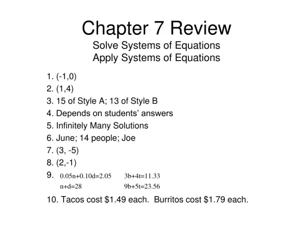
1 / 34
340 likes | 539 Views
Lecture 7 - Systems of Equations. CVEN 302 June 17, 2002. Lecture’s Goals. Discuss how to solve systems Gaussian Elimination Gaussian Elimination with Pivoting Tridiagonal Solver Problems with the technique Examples Iterative Techniques. Computer Program.

E N D
Lecture 7 - Systems of Equations CVEN 302 June 17, 2002
Lecture’s Goals • Discuss how to solve systems • Gaussian Elimination • Gaussian Elimination with Pivoting • Tridiagonal Solver • Problems with the technique • Examples • Iterative Techniques
Computer Program The program GEdemo(A,b) does the Gaussian elimination for a square matrix (nxn). It does not do any pivoting and works for only one {b} vector.
Test the Program • Example 1 • Example 2 • New Matrix 2X1 + 4X2 - 2 X3 - 2 X4 = - 4 1X1 + 2X2 + 4X3 - 3 X4 = 5 - 3X1 - 3X2 + 8X3 - 2X4 = 7 - X1 + X2 + 6X3 - 3X4 = 7
Problem with Gaussian Elimination • The problem can occur when a zero appears in the diagonal and makes a simple Gaussian elimination impossible. • Pivoting changes the matrix so that it will become diagonally dominate and reduce the round-off and truncation errors in the solving the matrix.
Example of Pivoting 2 X1 + 4 X2 - 2 X3 = 10 X1 + 2 X2 + 4 X3 = 6 2 X1 + 2 X2 + 1X3 = 2 Answer [X1 X2 X3 ] = [-3.40, 4.30, 0.20 ]
Computer Program • GEPivotdemo(A,b) is a program, which will do a Gaussian elimination on matrix A with pivoting technique to make matrix diagonally dominate. • The program is modification to handle a single value of {b}
Question? • How would you modify the programs to handle multiple inputs? • What is diagonal matrix, upper triangular matrix, and lower triangular matrix? • Can you do a column exchange and how would you handle the problem if it works?
Gaussian Elimination • If the diagonal is not dominate the problem can have round off error and truncation errors. • The scaling will result in problems
Question? • What happens with the following example? 0.0001X1 + 0.5 X2 = 0.5 0.4000X1 - 0.3 X2 = 0.1 • What happens is the second equation becomes: 0.4000X1 - 2000 X2 = -2000
Question? • What happens with the following example for values with two-significant figures? 0.4000 X1 - 0.3 X2 = 0.1 0.0001 X1 + 0.5 X2 = 0.5
Scaling • Scaling is an operation of adjusting the coefficients of a set of equations so that they are all of the same magnitude.
Scaling • A set of equations may involve relationships between quantities measured in a widely different units (N vs. kN, sec vs hrs, etc.) This may result in equation having very large number and others with very small , if we select pivoting may put numbers on the diagonal that are not large in comparison to other rows and create round-off errors that pivoting was suppose to avoid.
Scaling • What happens with the following example? 3X1 + 2 X2 +100X3 = 105 - X1 + 3 X2 +100X3 = 102 X1 + 2 X2 - 1X3 = 2
Scaling • The best way to handle the problem is to normalize the results. 0.03X1 + 0.02 X2 +1.00X3 = 1.05 - 0.01X1 + 0.03 X2 +1.00X3 = 1.02 0.50X1 +1.00 X2 - 0.50X3 = 1.00
Gauss-Jordan Method • The Gauss-Jordan Method is similar to the Gaussian Elimination. • The method requires almost 50% more operations.
Gauss-Jordan Method The Gauss-Jordan method changes the matrix into the identity matrix.
Gauss-Jordan Method There are one phases to the solving technique • Elimination --- use row operations to convert the matrix into an identity matrix. • The new b vector is the solution to the x values.
Gauss-Jordan Algorithm [A]{x} ={b} • Augment the n x n coefficient matrix with the vector of right hand sides to form a n x (n+1) • Interchange rows if necessary to make the value a11 with the largest magnitude of any coefficient in the first row • Create zero in 2nd through nth row in first row by subtracting ai1 /a11 times first row from ith row
Gauss-Jordan Elimination Algorithm • Repeat (2) & (3) for first through the nth rows, putting the largest magnitude coefficient in the diagonal by interchanging rows (consider only row j to n ) and then subtract times the jth row from the ith row so as to create zeros in all positions of jth column and the diagonal becomes all ones • Solve for all of the equations, xi = ai,n+1
Example 1 X1 + 3X2 = 5 2X1 + 4X2 = 6
Example 2 -3X1 + 2X2 - X3 = -1 6X1 - 6X2 + 7X3 = -7 3X1 - 4X2 + 4X3 = -6
Band Solver • Large matrices tend to be banded, which means that the matrix has a band of non-zero coefficients and zeroes on the outside of the matrix. • The simplest of the methods is the Thomas Method, which is used for a tridiagonal matrix.
Advantages of Band Solvers • The method reduce the number of operations and save the matrix in smaller amount of memory. • The band solver is faster and is useful for large scale matrices.
Thomas Method • The method takes advantage of the bandedness of the matrix. • The technique uses a two phase process. • The first phase is to obtain the coefficients from the sweep. • The second phase solves for the x values.
Thomas Method • The first phase starts with the first row of coefficients scales the a and r coefficients. • The second phase solves for x values using the a and r coefficients.
Thomas Method • The program for the method is given as demoThomas(a,d,b,r) • The algorithm is from the textbook, where a,d,b, & r are vectors from the matrix.
Iterative Techniques • The method of solving simultaneous linear algebraic equations using Gaussian Elimination and the Gauss-Jordan Method. These techniques are known as direct methods. Problems can arise from round-off errors and zero on the diagonal. • One means of obtaining an approximate solution to the equations is to use an “educated guess”.
Iterative Methods • We will look at three iterative methods: • Jacobi Method • Gauss-Seidel Method • Successive over Relaxation (SOR)
Convergence Restrictions • There are two conditions for the iterative method to converge. • Necessary that 1 coefficient in each equation is dominate. • The sufficient condition is that the diagonal is dominate.
Jacobi Iteration • If the diagonal is dominant, the matrix can be rewritten in the following form
Jacobi Iteration • The technique can be rewritten in a shorthand fashion, where D is the diagonal, A” is the matrix without the diagonal and c is the right-hand side of the equations.
Summary • Scaling of the problem will help in the convergence. • Gauss-Jordan method is more computational intense and does not improve the round-off errors. However, it is useful for finding matrix inverses. • Banded matrix solvers are faster and use less memory.
Homework • Check the Homework webpage