Download
1 / 19
200 likes | 550 Views
Matlab Fourier Analysis. 主講人:戴富隆. Item: Fourier Transform introduction 地震資料來源 使用指令 程式介紹. Fourier Transform introduction 傅立葉( Fourier, Jean Baptiste Joseph, 1768-1830 ) 十九世紀法國的數學家傅立葉發現了一個定理,即:任何的訊號(例如聲音、 影像等等)均可被拆解為頻率、振幅、相位角不等之正弦波的組合。. 傅立葉級數 :. 傅立葉複數轉換對 將信號由時間領域轉換到頻率領域

E N D
Matlab Fourier Analysis 主講人:戴富隆
Item: • Fourier Transform introduction • 地震資料來源 • 使用指令 • 程式介紹
Fourier Transform introduction • 傅立葉(Fourier, Jean Baptiste Joseph, 1768-1830) • 十九世紀法國的數學家傅立葉發現了一個定理,即:任何的訊號(例如聲音、 影像等等)均可被拆解為頻率、振幅、相位角不等之正弦波的組合。
傅立葉複數轉換對 將信號由時間領域轉換到頻率領域 F(ω) = ∫ f(x)exp(-jωx)dx F(x) =1/(2π) ∫ F(ω)exp(jωx)dω ∞ -∞ ∞ -∞
Discrete Fourier Transform X(k)= ∑ X(n) exp(-j2πnk/N) , for k=0…N-1 Inverse Discrete Fourier Transform X(n)=1/N ∑ X(k) exp(-j2πnk/N) , for n=0…N-1 幾乎在所有自然界的訊號(波動)都是連續的,但是在電腦世界的訊號,由於都是以位元為單位來儲存,所以這些訊號都是離散的,簡稱「離散時間訊號」(Discrete Time Signal) N-1 n=0 N-1 K=0
FFT (Fast Fourier Transform) Cooley and Tukey 於 1965提出FFT法 X(m)=1/N ∑ X(n)wmn , w= exp(-j2π/N) 將DFT由N^2複數乘法簡化成N*log2N/2複數乘法由N(N-1)複數加法簡化成N*log2N複數加法 N-1 n=0
3. 使用指令 fft: FFT(X) is the discrete Fourier transform (DFT) of vector X. For matrices, the FFT operation is applied to each column. angle: returns the phase angles, in radians, of a matrix with complex elements. phase angles = tan-1[I(f)/R(f)] , I(f)虛部 R(f)實部 angle(2+3i) = tan-1(3/2)= 0.9828
Subplot: creat axes in titled position SUBPLOT(m,n,p), or SUBPLOT(mnp), breaks the Figure window into an m-by-n matrix of small axes, selects the p-th axes for the current plot, and returns the axis handle. unwrap: unwraps radian phases P by changing absolute jumps greater than pi to their 2*pi complement. It unwraps along the first non-singleton dimension of P. P can be a scalar, vector, matrix, or N-D array.
figure: FIGURE(H) makes H the current figure, abs: ABS(X) is the absolute value of the elements of X.
4. 程式介紹 % StationCode: CHY080 %草嶺 % LocationLongitude(°E): 120.678 % LocationLatitude (°N): 23.597 % LocationElavation(M): 840.0 % InstrumentKind: A900A(T362002.263 ) % StartTime: 1999/ 9/20 17:47: 2.0 % SampleRate(Hz): 200 % AmplitudeUnit: gal % RecordLength(sec): 90.0 % DataSequence: U(+); N(+); E(+) % Data: 3F10.3
clear; N = 18000; % SampleRate(Hz): 200 * RecordLength(sec): 90 T = 1/200; %%1/SampleRate(Hz) k = 0:N-1; h = k*(1/(N*T)); % hertz load ch080.txt % 中央氣象局 921地震草嶺測站資料 ux = ch080(:,1)‘; % ch080.txt 第一行資料. ’ 轉為列 fu = fft(ux); up = unwrap(angle(fu)); figure(1);
%畫3列圖. % plot(0:T:T*(N-1),ux), x軸從0:T*(N-1), step T subplot(311);plot(0:T:T*(N-1),ux),ylabel('Amplitude (gal)'),xlabel('Time (s)'),grid on,title('921-草嶺sh080-Vertical component') subplot(312);plot(h(1:N),abs(fu)),ylabel('abs(FFT[Amp]])(gal)'),xlabel('Frequency (Hz)'),grid on subplot(313);plot(h(1:N),up),ylabel('Phase (rad)'),xlabel('Frequency (Hz)'),grid on
n = ch080(:,2)'; fn = fft(n); np = unwrap(angle(fn)); figure(2); subplot(311);plot(0:T:T*(N-1),n),ylabel('Amplitude (gal)'),xlabel('Time (s)'),grid on,title('921-草嶺sh080-NS component') subplot(312);plot(h(1:N),abs(fn)),ylabel('abs(FFT[Amp])(gal)'),xlabel('Frequency (Hz)'),grid on subplot(313);plot(h(1:N),np),ylabel('Phase (rad)'),xlabel('Frequency (Hz)'),grid on
e = ch080(:,3)'; fe = fft(e); ep = unwrap(angle(fe)); figure(3); subplot(311);plot(0:T:T*(N-1),e),ylabel('Amplitude (gal)'),xlabel('Time (s)'),grid on,title('921-草嶺sh080-EW component') subplot(312);plot(h(1:N),abs(fe)),ylabel('abs(FFT[Amp])(gal)'),xlabel('Frequency (Hz)'),grid on subplot(313);plot(h(1:N),ep),ylabel('Phase (rad)'),xlabel('Frequency (Hz)'),grid on