Download
1 / 90
910 likes | 1.2k Views
Solving Markov Random Fields using Second Order Cone Programming Relaxations. M. Pawan Kumar Philip Torr Andrew Zisserman. Aim. Accurate MAP estimation of pairwise Markov random fields. 0. 6. 1. 3. 2. 0. 4. Label ‘1’. 1. 2. 4. 1. 1. 3. Label ‘0’. 1. 0. 5. 0. 3. 7. 2.

E N D
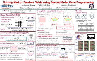
Solving Markov Random Fields using Second Order Cone Programming Relaxations M. Pawan Kumar Philip Torr Andrew Zisserman
Aim • Accurate MAP estimation of pairwise Markov random fields 0 6 1 3 2 0 4 Label ‘1’ 1 2 4 1 1 3 Label ‘0’ 1 0 5 0 3 7 2 V2 V3 V4 V1 Random Variables V = {V1,..,V4} Label Set L = {0,1} Labelling m = {1, 0, 0, 1}
Aim • Accurate MAP estimation of pairwise Markov random fields 0 6 1 3 2 0 4 Label ‘1’ 1 2 4 1 1 3 Label ‘0’ 1 0 5 0 3 7 2 V2 V3 V4 V1 Cost(m) = 2
Aim • Accurate MAP estimation of pairwise Markov random fields 0 6 1 3 2 0 4 Label ‘1’ 1 2 4 1 1 3 Label ‘0’ 1 0 5 0 3 7 2 V2 V3 V4 V1 Cost(m) = 2 + 1
Aim • Accurate MAP estimation of pairwise Markov random fields 0 6 1 3 2 0 4 Label ‘1’ 1 2 4 1 1 3 Label ‘0’ 1 0 5 0 3 7 2 V2 V3 V4 V1 Cost(m) = 2 + 1 + 2
Aim • Accurate MAP estimation of pairwise Markov random fields 0 6 1 3 2 0 4 Label ‘1’ 1 2 4 1 1 3 Label ‘0’ 1 0 5 0 3 7 2 V2 V3 V4 V1 Cost(m) = 2 + 1 + 2 + 1
Aim • Accurate MAP estimation of pairwise Markov random fields 0 6 1 3 2 0 4 Label ‘1’ 1 2 4 1 1 3 Label ‘0’ 1 0 5 0 3 7 2 V2 V3 V4 V1 Cost(m) = 2 + 1 + 2 + 1 + 3
Aim • Accurate MAP estimation of pairwise Markov random fields 0 6 1 3 2 0 4 Label ‘1’ 1 2 4 1 1 3 Label ‘0’ 1 0 5 0 3 7 2 V2 V3 V4 V1 Cost(m) = 2 + 1 + 2 + 1 + 3 + 1
Aim • Accurate MAP estimation of pairwise Markov random fields 0 6 1 3 2 0 4 Label ‘1’ 1 2 4 1 1 3 Label ‘0’ 1 0 5 0 3 7 2 V2 V3 V4 V1 Cost(m) = 2 + 1 + 2 + 1 + 3 + 1 + 3
Aim • Accurate MAP estimation of pairwise Markov random fields 0 6 1 3 2 0 4 Label ‘1’ 1 2 4 1 1 3 Label ‘0’ 1 0 5 0 3 7 2 V2 V3 V4 V1 Cost(m) = 2 + 1 + 2 + 1 + 3 + 1 + 3 = 13 Pr(m) exp(-Cost(m)) Minimum Cost Labelling = MAP estimate
Aim • Accurate MAP estimation of pairwise Markov random fields 0 6 1 3 2 0 4 Label ‘1’ 1 2 4 1 1 3 Label ‘0’ 1 0 5 0 3 7 2 V2 V3 V4 V1 Objectives • Applicable for all neighbourhood relationships • Applicable for all forms of pairwise costs • Guaranteed to converge
D C B G1 A D D C V1 C B B A A V2 V3 MRF G2 Motivation Subgraph Matching - Torr - 2003, Schellewald et al - 2005 Unary costs are uniform
G1 YES NO 2 1 G2 Potts Model Motivation Subgraph Matching - Torr - 2003, Schellewald et al - 2005 Pairwise Costs | d(mi,mj) - d(Vi,Vj) | <
D C B A D D C V1 C B B A A V2 V3 MRF Motivation Subgraph Matching - Torr - 2003, Schellewald et al - 2005
Motivation Subgraph Matching - Torr - 2003, Schellewald et al - 2005 D C B A D D C V1 C B B A A V2 V3 MRF
P2 (x,y,,) P1 P3 MRF Image Motivation Matching Pictorial Structures - Felzenszwalb et al - 2001 Outline Texture Part likelihood Spatial Prior
YES NO 2 1 P2 (x,y,,) P1 P3 MRF Image Motivation Matching Pictorial Structures - Felzenszwalb et al - 2001 • Unary potentials are negative log likelihoods Valid pairwise configuration Potts Model
YES NO 2 1 Motivation Matching Pictorial Structures - Felzenszwalb et al - 2001 • Unary potentials are negative log likelihoods Valid pairwise configuration Potts Model P2 (x,y,,) P1 P3 Image Pr(Cow)
Outline • Integer Programming Formulation • Previous Work • Our Approach • Second Order Cone Programming (SOCP) • SOCP Relaxation • Robust Truncated Model • Applications • Subgraph Matching • Pictorial Structures
Cost of V1 = 1 Cost of V1 = 0 Integer Programming Formulation 2 0 4 Unary Cost Label ‘1’ 1 3 Label ‘0’ 5 0 2 V2 V1 Labelling m = {1 , 0} ; 2 4 ] 2 Unary Cost Vector u = [ 5
V1= 1 V1 0 Integer Programming Formulation 2 0 4 Unary Cost Label ‘1’ 1 3 Label ‘0’ 5 0 2 V2 V1 Labelling m = {1 , 0} ; 2 4 ]T 2 Unary Cost Vector u = [ 5 Label vector x = [ -1 1 ; 1 -1 ]T Recall that the aim is to find the optimal x
Integer Programming Formulation 2 0 4 Unary Cost Label ‘1’ 1 3 Label ‘0’ 5 0 2 V2 V1 Labelling m = {1 , 0} ; 2 4 ]T 2 Unary Cost Vector u = [ 5 Label vector x = [ -1 1 ; 1 -1 ]T 1 Sum of Unary Costs = ∑iui (1 + xi) 2
Pairwise Cost Matrix P Cost of V1 = 0 and V1 = 0 0 Cost of V1 = 0 and V2 = 0 0 0 1 0 Cost of V1 = 0 and V2 = 1 0 1 0 0 3 0 0 0 Integer Programming Formulation 2 0 4 Pairwise Cost Label ‘1’ 1 3 Label ‘0’ 5 0 2 V2 V1 Labelling m = {1 , 0} 0 3 0
Pairwise Cost Matrix P 0 0 0 1 0 0 1 0 0 3 0 0 0 Integer Programming Formulation 2 0 4 Pairwise Cost Label ‘1’ 1 3 Label ‘0’ 5 0 2 V2 V1 Labelling m = {1 , 0} Sum of Pairwise Costs 1 ∑ijPij (1 + xi)(1+xj) 0 3 0 4
Pairwise Cost Matrix P 0 0 0 1 0 1 = ∑ijPij (1 + xi + xj + Xij) 4 0 1 0 0 3 0 0 0 Integer Programming Formulation 2 0 4 Pairwise Cost Label ‘1’ 1 3 Label ‘0’ 5 0 2 V2 V1 Labelling m = {1 , 0} Sum of Pairwise Costs 1 ∑ijPij (1 + xi +xj + xixj) 0 3 0 4 X = x xT Xij = xi xj
Each variable should be assigned a unique label ∑ xi = 2 - |L| i Va • Marginalization constraint ∑ Xij = (2 - |L|) xi j Vb Integer Programming Formulation Constraints
∑ xi = 2 - |L| i Va ∑ Xij = (2 - |L|) xi Convex Non-Convex j Vb Integer Programming Formulation Chekuri et al. , SODA 2001 1 1 ∑ Pij (1 + xi + xj + Xij) x* = argmin + ∑ ui (1 + xi) 4 2 xi{-1,1} X = x xT
Outline • Integer Programming Formulation • Previous Work • Our Approach • Second Order Cone Programming (SOCP) • SOCP Relaxation • Robust Truncated Model • Applications • Subgraph Matching • Pictorial Structures
Retain Convex Part ∑ xi = 2 - |L| i Va ∑ Xij = (2 - |L|) xi Relax Non-convex Constraint j Vb Linear Programming Formulation Chekuri et al. , SODA 2001 1 1 ∑ Pij (1 + xi + xj + Xij) x* = argmin + ∑ ui (1 + xi) 4 2 xi{-1,1} X = x xT
Retain Convex Part ∑ xi = 2 - |L| i Va ∑ Xij = (2 - |L|) xi Relax Non-convex Constraint j Vb Linear Programming Formulation Chekuri et al. , SODA 2001 1 1 ∑ Pij (1 + xi + xj + Xij) x* = argmin + ∑ ui (1 + xi) 4 2 xi[-1,1] X = x xT
Retain Convex Part ∑ xi = 2 - |L| i Va ∑ Xij = (2 - |L|) xi j Vb Linear Programming Formulation Chekuri et al. , SODA 2001 1 1 ∑ Pij (1 + xi + xj + Xij) x* = argmin + ∑ ui (1 + xi) 4 2 xi[-1,1]
Linear Programming Formulation x {-1,1}, X = x2 Feasible Region (IP)
Linear Programming Formulation x {-1,1}, X = x2 Feasible Region (IP) Feasible Region (Relaxation 1) x [-1,1], X = x2
Linear Programming Formulation x {-1,1}, X = x2 Feasible Region (IP) Feasible Region (Relaxation 1) x [-1,1], X = x2 Feasible Region (Relaxation 2) x [-1,1]
Linear Programming Formulation • Bounded algorithms proposed by Chekuri et al, SODA 2001 • -expansion - Komodakis and Tziritas, ICCV 2005 • TRW - Wainwright et al., NIPS 2002 • TRW-S - Kolmogorov, AISTATS 2005 • Efficient because it uses Linear Programming • Not accurate
Retain Convex Part ∑ xi = 2 - |L| i Va ∑ Xij = (2 - |L|) xi Relax Non-convex Constraint j Vb Semidefinite Programming Formulation Lovasz and Schrijver, SIAM Optimization, 1990 1 1 ∑ Pij (1 + xi + xj + Xij) x* = argmin + ∑ ui (1 + xi) 4 2 xi{-1,1} X = x xT
Retain Convex Part ∑ xi = 2 - |L| i Va ∑ Xij = (2 - |L|) xi Relax Non-convex Constraint j Vb Semidefinite Programming Formulation Lovasz and Schrijver, SIAM Optimization, 1990 1 1 ∑ Pij (1 + xi + xj + Xij) x* = argmin + ∑ ui (1 + xi) 4 2 xi[-1,1] X = x xT
Semidefinite Programming Formulation 1 xT = x X Convex Non-Convex . . . 1 1 x1 x2 xn x1 x2 . . . xn Xii = 1 Positive Semidefinite Rank = 1
Semidefinite Programming Formulation 1 xT = x X Convex . . . 1 1 x1 x2 xn x1 x2 . . . xn Xii = 1 Positive Semidefinite
0 I 0 A 0 I A-1B = BTA-1 0 0 I I C - BTA-1B A 0 C -BTA-1B 0 Schur’s Complement A B BT C
Semidefinite Programming Formulation 1 0 1 0 I xT = x 0 0 I X - xxT 1 Schur’s Complement X - xxT 0 1 xT x X
Retain Convex Part ∑ xi = 2 - |L| i Va ∑ Xij = (2 - |L|) xi Relax Non-convex Constraint j Vb Semidefinite Programming Formulation Lovasz and Schrijver, SIAM Optimization, 1990 1 1 ∑ Pij (1 + xi + xj + Xij) x* = argmin + ∑ ui (1 + xi) 4 2 xi[-1,1] X = x xT
Retain Convex Part ∑ xi = 2 - |L| i Va ∑ Xij = (2 - |L|) xi j Vb X - xxT 0 Semidefinite Programming Formulation Lovasz and Schrijver, SIAM Optimization, 1990 1 1 ∑ Pij (1 + xi + xj + Xij) x* = argmin + ∑ ui (1 + xi) 4 2 xi[-1,1] Xii = 1
Semidefinite Programming Formulation x {-1,1}, X = x2 Feasible Region (IP)
Semidefinite Programming Formulation x {-1,1}, X = x2 Feasible Region (IP) Feasible Region (Relaxation 1) x [-1,1], X = x2
Semidefinite Programming Formulation x {-1,1}, X = x2 Feasible Region (IP) Feasible Region (Relaxation 1) x [-1,1], X = x2 Feasible Region (Relaxation 2) x [-1,1], X x2
Semidefinite Programming Formulation • Formulated by Lovasz and Schrijver, 1990 • Finds a full X matrix • Max-cut - Goemans and Williamson, JACM 1995 • Max-k-cut - de Klerk et al, 2000 • Accurate • Not efficient because of Semidefinite Programming
Previous Work - Overview Is there a Middle Path ???
Outline • Integer Programming Formulation • Previous Work • Our Approach • Second Order Cone Programming (SOCP) • SOCP Relaxation • Robust Truncated Model • Applications • Subgraph Matching • Pictorial Structures
x2 + y2 z2 Second Order Cone Programming Second Order Cone || v || t OR || v ||2 st