Download
1 / 83
830 likes | 988 Views
Skin. CSE169: Computer Animation Instructor: Steve Rotenberg UCSD, Winter 2004. Computer Lab. Lab: AP&M 2444 Combo: 0562340 Turning in: Place all files in a .zip file with your name: example: ‘steve_rotenberg_project1’

E N D
Skin CSE169: Computer Animation Instructor: Steve Rotenberg UCSD, Winter 2004
Computer Lab • Lab: AP&M 2444 • Combo: 0562340 • Turning in: • Place all files in a .zip file with your name: example: ‘steve_rotenberg_project1’ • Include all necessary files (.cpp, .h, .dsp & .dsw on Windows, makefile on Linux…) • Include ‘readme.txt’ with any other relevant information (problems, additional features, keyboard controls…) • Use ‘turnin’
Project 1 • Please make the program take an optional .skel file name as a command line parameter. If no file name is specified, it should default to test.skel • Feel free to pass argc, argv to Tester::Tester() and to simplify Token::Open() to take just an entire file name • Grading: 15 points
Extra Credit (Project 1) • Make your own .skel file with 10 or more joints and pose it. Use DOF limits, various box sizes, offsets, and a non-trivial tree (no snakes!). 1 point. • Add an interactive interface to the skeleton program. Allow the user to select a DOF with the mouse (either by picking or from a list) and adjust the value interactively. Display the selected DOF name and value on the screen. 2 points.
Recommended Reading • “3-D Computer Graphics: A Mathematical Introduction with OpenGL” (Buss) • Appendix A: Vectors • Chapter 2: Transformations and Viewing • Chapter 12: Animation and Kinematics • “Pose-Space Deformation: A Unified Approach to Shape Interpolation and Skeleton Driven Deformation” (Lewis, Cordner, Fong) • “Skinning Characters Using Surface Oriented Free Form Deformations” (Singh, Kokkevis)
Example: Target ‘Lock On’ • For an airplane to get a missile locked on, the target must be within a 10 degree cone in front of the plane. If the plane’s matrix is M and the target position is t, find an expression that determines if the plane can get a lock on. b • t d c a
Example: Target ‘Lock On’ • We want to check the angle between the heading vector (-c) and the vector from d to t: • We can speed that up by comparing the cosine instead ( cos(10°)=.985 )
Example: Target ‘Lock On’ • We can even speed that up further by removing the division and the square root in the magnitude computation:
Orthonormality • If all row vectors and all column vectors of a matrix are unit length, that matrix is said to be orthonormal • This also implies that all vectors are perpendicular to each other • Orthonormal matrices have some useful mathematical properties, such as: • M-1 = MT
Orthonormality • If a 4x4 matrix represents a rigid transformation, then the upper 3x3 portion will be orthonormal
Determinants • The determinant of a 4x4 matrix with no projection is equal to the determinant of the upper 3x3 portion
Determinants • The determinant is a scalar value that represents the volume change that the transformation will cause • An orthonormal matrix will have a determinant of 1, but non-orthonormal volume preserving matrices will have a determinant of 1 also • A flattened or degenerate matrix has a determinant of 0 • A matrix that has been mirrored will have a negative determinant
Matrix Transformations • We usually transform vertices from some local space where they are defined into a world space v’ = v·W • Once in world space, we can perform operations that require everything to be in the same space (collision detection, high quality lighting…) • Then, they are transformed into a camera’s space, and then projected into 2D v’’ = v’·C-1·P • In simple situations, we can do this all in one step: v’’ = v·W·C-1·P
Camera Matrix • Think of the camera just like any other object. Just as a chair model has a matrix W that transforms it into world space, the camera matrix C would transform a camera model into world space. • We don’t want to transform the camera into world space. Instead, we want to transform the world into the camera’s space, so we use the inverse of C.
Example: Camera ‘Look At’ • Our eye is located at position e and we want to look at a target at position t. Generate an appropriate camera matrix M.
Example: Camera ‘Look At’ • Our eye is located at position e and we want to look at a target at position t. Generate an appropriate camera matrix M. • Two possible approaches include: • Measure angles and rotate matrix into place • Construct a,b,c, & d vectors of M directly
Example: Camera ‘Look At’Method 1: Measure Angles & Rotate • Measure Angles: • Tilt angle • Heading angle • Position • Construct matrix
Example: Camera ‘Look At’Method 2: Build Matrix Directly • The d vector is just the position of the camera, which is e: • The c vector is a unit length vector that points directly behind the viewer:
Example: Camera ‘Look At’Method 2: Build Matrix Directly • The a vector is a unit length vector that points to the right of the viewer. It is perpendicular to the c axis. To keep the camera from rolling, we also want the a vector to lay flat in the xz-plane, perpendicular to the y-axis. • Note that a cross product with the y-axis can be optimized as follows:
Example: Camera ‘Look At’Method 2: Build Matrix Directly • The b vector is a unit length vector that points up relative to the viewer. It is perpendicular to the both the c and a axes • Note that b does not need to be normalized because it is already unit length. This is because a and c are unit length vectors 90 degrees apart.
Example: Camera ‘Look At’Method 2: Build Matrix Directly • Summary:
Rendering • Renderable surfaces are built up from simple primitives such as triangles • They can also use smooth surfaces such as NURBS or subdivision surfaces, but these are often just turned into triangles by an automatic tessellation algorithm before rendering
Lighting • We can compute the interaction of light with surfaces to achieve realistic shading • For lighting computations, we usually require a position on the surface and the normal • GL does some relatively simple local illumination computations • For higher quality images, we can compute global illumination, where complete light interaction is computed within an environment to achieve effects like shadows, reflections, caustics, and diffuse bounced light
Gouraud & Phong Shading • We can use triangles to give the appearance of a smooth surface by faking the normals a little • Gouraud shading is a technique where we compute the lighting at each vertex and interpolate the resulting color across the triangle • Phong shading is more expensive and interpolates the normal across the triangle and recomputes the lighting for every pixel
Materials • When an incoming beam of light hits a surface, it will some of the light will be absorbed, and some will scatter in various directions
Materials • In high quality rendering, we use a function called a BRDF (bidirectional reflectance distribution function) to represent the scattering of light at the surface: fr(θi, φi, θr, φr, λ) • The BRDF is a 5 dimensional function of the incoming light direction (2 dimensions), the outgoing direction (2 dimensions), and the wavelength
Translucency • Skin is a translucent material. If we want to render skin realistically, we need to account for subsurface light scattering. • We can extend the BRDF to a BSSRDF by adding two more dimensions representing the translation in surface coordinates. This way, we can account for light that enters the surface at one location and leaves at another. • Learn more about these in CSE168!
Rigid Parts • Robots and mechanical creatures can usually be rendered with rigid parts and don’t require a smooth skin • To render rigid parts, each part is transformed by its joint matrix independently • In this situation, every vertex of the character’s geometry is transformed by exactly one matrix where v is defined in joint’s local space
Simple Skin • A simple improvement for low-medium quality characters is to rigidly bind a skin to the skeleton. This means that every vertex of the continuous skin mesh is attached to a joint. • In this method, as with rigid parts, every vertex is transformed exactly once and should therefore have similar performance to rendering with rigid parts.
Smooth Skin • With the smooth skin algorithm, a vertex can be attached to more than one joint with adjustable weights that control how much each joint affects it • Verts rarely need to be attached to more than three joints • Each vertex is transformed a few times and the results are blended • The smooth skin algorithm has many other names: blended skin, skeletal subspace deformation (SSD), multi-matrix skin, matrix palette skinning…
Smooth Skin Algorithm • The deformed vertex position is a weighted sum:
Binding Matrices • With rigid parts or simple skin, v can be defined local to the joint that transforms it • With smooth skin, several joints transform a vertex, but it can’t be defined local to all of them • Instead, we must first transform it to be local to the joint that will then transform it to the world • To do this, we use a binding matrix B for each joint that defines where the joint was when the skin was attached and premultiply its inverse with the world matrix:
Normals • To compute shading, we need to transform the normals to world space also • Because the normal is a direction vector, we don’t want it to get the translation from the matrix, so we only need to multiply the normal by the upper 3x3 portion of the matrix • For a normal bound to only one joint:
Normals • For smooth skin, we must blend the normal as with the positions, but the normal must then be renormalized: • If the matrices have non-rigid transformations, then technically, we should use:
Algorithm Overview Skin::Update() (view independent processing) • Compute skinning matrix for each joint: M=B-1·W (you can precompute and store B-1 instead of B) • Loop through vertices and compute blended position & normal Skin::Draw() (view dependent processing) • Set matrix state to Identity (world) • Loop through triangles and draw using world space positions & normals Questions: • Why not deal with B in Skeleton::Update() ? • Why not just transform vertices within Skin::Draw() ?
Muscles & Other Effects • One can add custom effects such as muscle bulges as additional joints • For example, the bicep could be a translational or scaling joint that smoothly controls some of the verts in the upper arm. Its motion could be linked to the motion of the elbow rotation. • With this approach, one can also use skin for muscles, fat bulges, facial expressions, and even simple clothing
Limitations of Smooth Skin • Smooth skin is very simple and quite fast, but its quality is limited • The main problems are: • Joints tend to collapse as they bend more • Very difficult to get specific control • Unintuitive and difficult to edit • Still, it is built in to most 3D animation packages and has support in both OpenGL and Direct3D • If nothing else, it is a good baseline upon which more complex schemes can be built
Bone Links • To help with the collapsing joint problem, one option is to use bone links • Bone links are extra joints inserted in the skeleton to assist with the skinning • They can be automatically added based on the joint’s range of motion. For example, they could be added so as to prevent any joint from rotating more than 60 degrees. • This is a simple approach used in some real time games, but doesn’t go very far in fixing the other problems with smooth skin.
Shape Interpolation • Another extension to the smooth skinning algorithm is to allow the verts to be modeled at key values along the joints motion • For an elbow, for example, one could model it straight, then model it fully bent • These shapes are interpolated local to the bones before the skinning is applied • We will talk more about this technique in the next lecture
Rigging Process • To rig a skinned character, one must have a geometric skin mesh and a skeleton • Usually, the skin is built in a relatively neutral pose, often in a comfortable standing pose • The skeleton, however, might be built in more of a ‘zero’ pose where are joints DOFs are assumed to be 0, causing a very stiff, straight pose • To attach the skin to the skeleton, the skeleton must first be posed into a binding pose • Once this is done, the verts can be assigned to joints with appropriate weights
Skin Binding • Attaching a skin to a skeleton is not a trivial problem and usually requires automated tools combined with extensive interactive tuning • Binding algorithms typically involve heuristic approaches • Some general approaches: • Containment • Point-to-line mapping • Delaunay tetrahedralization
Containment Binding • With containment binding algorithms, the user manually approximates the body with volume primitives for each bone (cylinders, ellipsoids, spheres…) • The algorithm then tests each vertex against the volumes and attaches it to the best fitting bone • Some containment algorithms attach to only one bone and then use smoothing as a second pass. Others attach to multiple bones directly and set skin weights • For a more automated version, the volumes could be initially set based on the bone lengths and child locations
Point-to-Line Mapping • A simple way to attach a skin is treat each bone as one or more line segments and attach each vertex to the nearest line segment • A bone is made from line segments connecting the joint pivot to the pivots of each child
Delaunay Tetrahedralization • This tricky computational geometry technique builds a tetrahedralization of the volume within the skin • The tetrahedra connect all of the skin verts and skeletal pivots in a relatively clean ‘Delaunay’ fashion • The connectivity of the mesh can then be analyzed to determine the best attachment for each vertex
Skin Adjustment • Mesh Smoothing: A joint will first be attached in a fairly rigid fashion (either automatic or manually) and then the weights are smoothed algorithmically • Rogue Removal: Automatic identification and removal of isolated vertex attachments • Weight Painting: Some 3D tools allow visualization of the weights as colors (0…1 -> black…white). These can then be adjusted and ‘painted’ in an interactive fashion • Direct Manipulation: These algorithms allow the vertex to be moved to a ‘correct’ position after the bone is bent, and automatically compute the weights necessary to get it there