Download
1 / 60
600 likes | 613 Views
Adjusting Highway Mileage in 3-D Using LIDAR. By Hubo Cai August 4 th , 2004. Organization. Introduction Research Objectives 3-D Models and 3-D Distance Prediction Computational Implementations Case Study Accuracy Evaluation and Sensitivity Analysis Significant Factors

E N D
Adjusting Highway Mileage in 3-D Using LIDAR By Hubo Cai August 4th, 2004
Organization • Introduction • Research Objectives • 3-D Models and 3-D Distance Prediction • Computational Implementations • Case Study • Accuracy Evaluation and Sensitivity Analysis • Significant Factors • Conclusions and Recommendations
Introduction • Why adjust highway mileage? • Location is Critical in Transportation • Events Are Located via Distances along Roads to Reference Points • Errors and Inconsistencies in Distance Measures in Transportation Spatial Databases • Why use GIS? • Other methods • Design Drawings • Ground Surveying • GPS • Distance Measurement Instrument (DMI) • Time-consuming and labor intensive • GIS-based approach is efficient
Introduction (Continued) • Why in 3-D? • Real World Objects ---- Three Dimensional • Using 2-D Length • Why LIDAR? • 3-D approach (the introduction of elevation) • Highly accurate • Availability • Main concerns • How? • Accuracy and error propagation
Research Objectives • Adjust highway mileage in 3-D using LIDAR • Evaluate its accuracy via a case study • Evaluate its sensitivity to the use of LIDAR versus NED • Identify significant factors
3-D Models • 3-D Point Model and Its Variants • 3-D Distance Prediction
3-D Point Model Specified by Z = f31 (X, Y) and Y = f3(X) Specified by Z = f2 (X, Y) and Y = f2(X) Z Specified by Z = f1 (X, Y) and Y = f1(X) F G B C E D A X F A B G E C D Y Specified by Y = f3 (X) Specified by Y = f1 (X) Specified by Y = f2 (X)
3-D Point Model – Variant 1, LRS-Based Specified by Z = f3 (Distance) Specified by Z = f2 (Distance) F Specified by Z = f1 (Distance) G E C D B Z/Elevation A LRS Distance Y 2-D Line F D G B C E A X
3-D Point Model – Variant 2, LRS-Based Straight Line Segments F G B E C D Z/Elevation A LRS Distance Y 2-D Line F D G B C E A X
Difference in Elevation--d Planimetric Length--pl 3-D Distance Prediction Surface Length = sqrt (d*d + pl*pl) Vertical Profile Horizon Horizontal Projection
Required Source Data • Elevation Dataset • LIDAR • USGS NED • Planimetric Line Dataset
LIDAR • General Information • A LIDAR operates in the Ultraviolet, Visible, and Infrared Region of the Electromagnetic Spectrum • A LIDAR consists of GPS, INS/IMU, and Laser Range Finder • Last “return” for Bare Earth Data • Raw Data – Mass Point Data • End Products Generation • Post Processing • Comma-Delimited ASCII File in X/Y/Z Format • DEMs • Accuracy • A Typical 6-Inch Error Budget in Elevations and Positions • The Guaranteed Best Vertical Accuracy -- ± 6 Inches (± 15 Centimeters) • No Better than 4 Inches • Market Models – Range from 10 – 30 cm (Vertical RMSE)
Column 0 1 2 4 5 3 0 1 2 Row 3 4 X, Y coordinates are (4, 3) DEMs • A DEM is a digital file consisting of terrain elevations for ground positions at regularly spaced horizontal intervals • Grid Surface
NED • Future Direction of USGS DEM Data • Merge the Highest-Resolution, Best-Quality Elevation Data Available across the US into a Seamless Raster Format • Source Data Selected According to the Following Criteria (Ordered from First to Last): 10-Meter DEM, 30-Meter Level-2 DEM, 30-Meter Level-1 DEM, 2-Arc-Second DEM, 3-Arc-Second DEM • Accuracy • Varies with Source Data • Systematic Evaluation under Processing • “Inherits” the Accuracy of the Source Data • Level 1 DEMs (Max RMSE 15 m, Desired RMSE 7 m) • Level 2 DEMs (Max RMSE One-half Contour Interval) • Level 3 DEMs (Max RMSE One-third Contour Interval)
Computational Implementations • Development Environments • ArcGIS 8.2 • ArcObjects • Visual Basic for Applications • Key ---- Obtaining 3-D Points • Obtaining Planimetric Positions (Depending on the Format of Input Elevation Data) • Obtaining Elevations
Obtaining 3-D Points ---- Working with LIDAR Points • Working with LIDAR Point Data • Depending on the Point Elevation Data • Interpolation Approach • Approximation Approach • Discussions
Interpolation Approach Group A points Group C points • Apply A Buffer • Identify All Points in the Buffer • Group Points into 3 Groups • Use Group C Points Directly • Identify Point Pairs for Group A and Group B Points • Create Points from Each Point Pair by Linear Interpolation • Deal with Start and End Points Group B points Elevation for point O is linearly interpolated from points P and Q P O Q
Approximation Approach • Developed based on Road Geometry • Apply A Buffer • Identify All Points in the Buffer • Points on Line for Direct Use • Snap Points to the Line • Deal with Start and End Points
Discussion Vertical error due to approximation • Errors due to Approximation • Typical Lane Width (12 ft for Interstate and US Roads, 10 ft for NC Routes) • Typical Cross-Sectional Slope (2%) • Maximum Errors based on the typical slope (0.24 ft ( 7.31cm) and 0.2 ft (6.10 cm)) • Prerequisite • Lines in Correct Positions • High-Density LIDAR Points • LIDAR Point Density • 18.6 ft (Average Distance between Two Neighboring LIDAR Points) • Discussion • Approximation Approach Results in Almost Double the Number of 3-D Points • Snapping Provides At Least Equal Accuracy, If Not Better Vertical error due to interpolation Points after Snapping Corresponding point on road centerline C LIDAR point A B B C A A LIDAR point B
30m C B 1035 1048 22.4m C B 30m 1041 1060 22.25m E G D A E F D A 1056.98 1052.46 1039.49 d B D d d A C Obtaining 3-D Points ---- Working with LIDAR DEMs and NED • Planimetric Position (2-D Point) ---- Uniform Interval (full cell-size and half cell-size) • Elevation • For A Given Point, Its Elevation Is Interpolated from Elevations of the Four Surrounding Cells • Two Steps (Intermediate Points and the Target Point)
Case Study ---- Study Scope • Limited by LIDAR Availability • Considered Sample Size and Variety • Interstate Highways in 9 Counties and US and NC Routes in Johnston County Study Scope TAR-PAMLICO NEUSE Legend River Basin County Counties in Study Scope Interstate Highways Map produced by Hubo Cai, August 2003 US Routes NC Routes
Case Study Information Sources • Digital Road Centerline Data • Elevation Data • LIDAR Point Data • LIDAR DEMs (20 and 50 ft resolutions) • NED (30 m resolution) • Reference Data (DMI Data)
Digital Road Centerline Data • Digitized from DOQQs ---- 93 B/W and 98 CIR • Data Description • Link-Node Format • County by County • Stateplane Coordinate System • Datum: NAD83 • Units: foot
Elevation Data – LIDAR Data • Data Collection and Description • Downloaded from www.ncfloodmaps.com • Tile by Tile (10,000 ft * 10, 000 ft) • Bare Earth Point Data, 20-ft DEMs, and 50-ft DEMs (ASCII Files) • Datum: NAD83 and NAVD 88 • Units: Foot • Accuracy • Coastal Counties (95% RMSE, 20 cm) • Inland Counties (95% RMSE, 25 cm) • Metadata States: 2 m Horizontal, 25 cm Vertical
Elevation Data -- NED • Data Collection and Description • Downloaded from North Carolina State University Spatial Information Lab (http://www.precisionag.ncsu.edu/) • County by County • Interchange Files (.e00 Files) • Stateplane Coordinate System • Datums: NAD83 and NAVD88 • Units: Foot (Horizontal), Meter (Vertical) • Resolution: 1-arc-second (approximately 30-Meter or 92.02-Feet) • Errors and Accuracy • Inherits the Accuracy of the Source DEMs • Metadata States Source DEMs Are Level 1 DEMs • Vertical RMSE: 7-Meter (Desired), 15-Meter (Maximum)
Modeling Road Centerlines in 3-D • Using LIDAR Point Data • Intermediate Points (Buffering and Snapping) • Start and End Points (Interpolation, Extrapolation, and Weighted Average) • Using LIDAR DEMs • Uniformly Distributed Points • Intervals • 20-ft and 10-ft with 20-ft DEMs • 50-ft and 25-ft with 50-ft DEMs • Using NED • Same as Using LIDAR DEMs • Different Intervals (30-meter and 15-meter)
Quality Control Points do not Follow the general trend
A Typical Scenario Bridge Buffer Buffer F4 L4 E4 Buffer Buffer P1/P2 L3 E3 D6 D5 D1 D2 F2 D4 F1 D3 L2 E2 Buffer L1 Buffer E1 Buffer F3 Buffer Bridge
Improvement D1 A1 • An Averaging Procedure • Averaging Criteria • Based on Average Densities • 3 ft for Interstate and US FTSegs (average density 9.69 ft) • 4 ft for NC FTSegs (average density 10.92 ft) L3 D3 L1 D4 L2 L4 A2 D2
Results • Each Road Segment Has 8 Distances • Predicted 3-D Distance • From the Use of LIDAR Point Data • From the Use of LIDAR 20-ft DEMs and A 10-ft Interval • From the Use of LIDAR 20-ft DEMs and A 20-ft Interval • From the Use of LIDAR 50-ft DEMs and A 25-ft Interval • From the Use of LIDAR 50-ft DEMs and A 50-ft Interval • From the Use of NED and A 15-m Interval • From the Use of NED and A 30-m Interval • Reference Distance • DMI Measured Distance
Accuracy Evaluation • Error(Difference) and Proportional Error (Proportional Difference) • Evaluation Methods • Descriptive Statistics (Describing Samples) • Distribution Histograms • Statistical Inferences • Frequency Analysis • 100% and 95% RMSEs • Sensitivity Analysis • Analysis of Variance (ANOVA) • Comparison of Means, Medians, Absolute Means, Frequencies, and RMSEs
Accuracy Evaluation Results ---- Hypothesis Tests and Confidence Intervals
Accuracy Evaluation Results ---- Frequency Analysis (LIDAR Point Data)
Sensitivity Analysis ---- ANOVA Difference: F > Fc, Proportional Difference: F < Fc
Conclusions ---- Accuracy Evaluation and Sensitivity Analysis • Errors of the predicted 3-D distances are not normally distributed. • The higher the accuracy of the elevation dataset being used, the higher the accuracy of the predicted 3-D distances. • Using the same elevation dataset, the accuracy of the predicted 3-D distance is not dependent on intervals, given these intervals are less than or equal to the cell size. • 3-D distances predicted using LIDAR point data with the snapping approach have the best accuracy.
Conclusions ---- Accuracy Evaluation and Sensitivity Analysis (Continued) • From the aspect of differences using the 100% RMSE as the measure of the accuracy, the use of LIDAR point data improves the accuracy by 28% compared to the use of NED data. The use of LIDAR DEMs improves the accuracy by 6% compared to the use of NED data. • From the aspect of differences using the 95% RMSE as the measure of the accuracy, the use of LIDAR point data improves the accuracy by 25% compared to the use of NED data. The use of LIDAR DEMs improves the accuracy by 8% compared to the use of NED data. • From the aspect of proportional differences, the improvements due to the use of higher accurate elevation datasets are not significant (the majority (53%) of the road segments in this case study are longer than 5,000 ft, 73% are longer than 1,000 ft, and 43% are longer than 10,000 ft).
Significant Factors • Goal • Evaluate the relationship between a geometric property and the accuracy of the GIS calculated distance • Factors under Consideration • Distance • Average Slope and Weighted Slope • Average Slope Change and Weighted Slope Change • Number of 3-D Points and Average Density of 3-D Points • Evaluation Methods Applied • Sample Correlation Coefficient and Sample Coefficient of Determination • Grouping and Comparison • Benefits • Cautions to be paid to certain linear features
Calculation of Factors • Distance = D1 + D2 (DMI measured) • Average Slope = (Abs(S1) + Abs(S2))/2 • Weighted Slope = (Abs(S1) * D1 + Abs(S2) * D2)/(D1 + D2) • Average Slope Change = (Abs(S1 – 0) + Abs(S2 – S1))/2 • Weighted Slope Change = (Abs(S1 – 0) * D1 + Abs(S2 – S1) * D2)/(D1 + D2) • Number of 3-D Points = 3 • Average Density = (D1 + D2)/2 D2 E2 S2 D1 E1 S1 PD1 PD2
Evaluation Result I: Distance vs. Difference and Absolute Difference Distance vs. Difference Distance vs. Absolute Difference
Grouping and Analysis I: Difference, Groups Based on Distance
Grouping and Analysis II: Proportional Difference, Groups Based on Distance
Significant Factor ---- Conclusions • Conclusions Based on Sample Correlation Coefficients • The Factors under Consideration are all significant to the accuracy of the predicted 3-D Distance when compared to the DMI measured distance. • Positive Linear Association between the error of the predicted 3-D distance and a factor under consideration. • Negative Linear Association between the proportional error of the predicted 3-D distance and a factor under consideration • Conclusions Based on Grouping and Analysis • Confirms the significance of these factors • Confirms the general linear associations • Reveals the existence of thresholds
Conclusions • It is technically feasible to model linear objects in a 3-D space with existing datasets. • The buffering and snapping approach is a creative way in using LIDAR point data. • Two datasets (elevation and line) are required to adopt the model developed. • The prerequisite to adopt the developed 3-D model is that lines are in correct positions. • Using the proposed 3-D approach, geometric properties other than 3-D distance could be calculated. • Conclusions regarding accuracy and sensitivity. • Conclusions regarding significant factors.