Download
1 / 29
290 likes | 486 Views
Design of Disturbance Rejection Controllers for a Magnetic Suspension System. By: Jon Dunlap Advisor: Dr. Winfred K.N. Anakwa Bradley University April 27, 2006. Outline Of Presentation: . Goal System Information Previous Lab Work Preliminary Lab Work Internal Model Principle

E N D
Design of Disturbance Rejection Controllers for a Magnetic Suspension System By: Jon Dunlap Advisor: Dr. Winfred K.N. Anakwa Bradley University April 27, 2006
Outline Of Presentation: • Goal • System Information • Previous Lab Work • Preliminary Lab Work • Internal Model Principle • Design Process • Results • Conclusion
Multiple Controllers for Multiple Disturbances Digital Controllers Created In Simulink xPC Target Box Serving as “Controller Container” Minimize Steady-State Error, Overshoot and Setting Time Act As A Stepping Stone From Previous Work Practical Use in Antenna Stabilization Goal
Method • Method of Choice: • Internal Model Principle • B.A. Francis & W.M. Wonham • The Internal Model Principle of Control Theory, 1976 • Chi-Tsong Chen • Linear System Theory and Design, 3rd, 1999 • Analogous to an Umbrella
Functional Description • Host PC using Simulink and xPC software • xPC Target Box with Controllers • Magnetic Suspension System • Feedback Incorporated 33-210
Previous Lab Work • Using Classical Controller • Will It Reject Disturbances?
Previous Lab Work • Results of Classical Controller With Disturbance • Rejected Step Disturbance
Preliminary Lab Work • Laplace Transfer Functions Found • Later Converted To Discrete Using Zero-order Hold
Internal Model Principle • Uses a Model to Cancel Unstable Poles of Reference and Disturbance Inputs to Provide Asymptotic Tracking and Disturbance Rejection • Model Is: Least Common Multiple of Unstable or Zero Continuous Denominator Poles • Ramp Disturbance Input = 0,0 • Step Reference Input = 0 • Model = P = 0,0
Design Approach • Disturbance Removed – Model Inserted • Must Stabilize Plant at all Times • Disturbance Should Never Affect Plant Output • 3 Known, 2 Unknown • A(z)D(z)P(z) + B(z)N(z)
Diophantine Equation • A(z)D(z)P(z) + B(z)N(z) = F(z) • Want: • Choose Poles to Form F Polynomial • Discrete, Close to 1 • Need: • Order of Controller • Order of D(z)P(z) – 1 = Order of Controller • Order of F • 2*(Order of D(z)P(z))-1 = Order of F
Keep In Mind - Account for Model when Implementing Controller • Controller Order Assumes Denominator without Model • Adding Model Increases Order Beyond Designed Value • Ex. If D(z)P(z)=4, then Controller=3 • But Model=2 so Controller Denominator really should be 1
Pole Placement • Ideal Situation • Tsettle = 60ms • %O.S. = 18 • = .479 • Wn= • Wn= 139.1788 • Wn<
Pole Placement Problems and Solution • Complex Poles Give Oscillations • Wn < Poles>.92 • All Poles Close To 1 Is Too Slow • Speed Up With Poles Closer To Origin • Iterative Design Approach Required • Working Poles For Ramp Rejection At: .9947, .9716, .9275, .9, .01 F(z) =
Diophantine Solution • A(z)D(z)P(z) + B(z)N(z) = F(z) • Combine D(z)P(z) to Equal D*(z) • For Each X(z)= • System of Equations To Be Solved Simultaneously • A0D*0+B0N0=F0…AnD*n+BnNn=Fn
Diophantine Solution • Using Previous Example:
Actual Values For Ramp Controller • N(z) = • D(z) = • P(z) = • F(z) = • B(z) = • A(z) = • A(z)P(z) =
Results – Stability • 2V Step Disturbance at 2.00V Set Point • 5V/s Ramp Disturbance at 2.00V Set Point 2.042 2.042
Results – Tracking • 5V/s Ramp Disturbance 6Hz .5V Peak-Peak Sine Wave Input 5.98Hz .7V Peak-Peak Sine Wave Output
Conclusion • Problems • Simulation Does Not Match Plant • Pole Locations are Hard to Find • <300mV Error at Start Up • Future • Continue to Implement Sinusoidal and Square Wave • Fine Tune Ramp With Better Poles
Control and Disturbance Signal Create Current Current Induces Magnetic Field Field Suspends Ball Sensor Translates Location into Voltage Magnetic Suspension System
xPC Target Box and Host PC • Using ±10 V ADC and DAC • Host Uploads Controller and Commands • Process Position Data and Passes Control
Modeling Hybrid Systems “Simulink treats any model that has both continuous and discrete sample times as a hybrid model, presuming that the model has both continuous and discrete states. Solving such a model entails choosing a step size that satisfies both the precision constraint on the continuous state integration and the sample time hit constraint on the discrete states. Simulink meets this requirement by passing the next sample time hit, as determined by the discrete solver, as an additional constraint on the continuous solver. The continuous solver must choose a step size that advances the simulation up to but not beyond the time of the next sample time hit. The continuous solver can take a time step short of the next sample time hit to meet its accuracy constraint but it cannot take a step beyond the next sample time hit even if its accuracy constraint allows it to.” http://www.mathworks.com/access/helpdesk/help/toolbox/simulink/ug/f7-23387.html