Download
1 / 80
950 likes | 1.45k Views
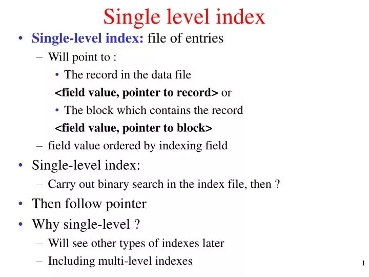
Single level index. Single-level index: file of entries Will point to : The record in the data file <field value, pointer to record> or The block which contains the record <field value, pointer to block> field value ordered by indexing field Single-level index:

E N D
Single level index Single-level index: file of entries Will point to : The record in the data file <field value, pointer to record> or The block which contains the record <field value, pointer to block> field value ordered by indexing field Single-level index: Carry out binary search in the index file, then ? Then follow pointer Why single-level ? Will see other types of indexes later Including multi-level indexes 1
Types of Single-Level Indexes: Primary Index Defined on data file ordered on a key field We will think of as Primary Key Indexing field will also be ordered by same key One index entry for each block in data file the index entry has the key field value for the first record in the block called the block anchor Dense or sparse ? Sparse : includes an entry for each disk block Not for every record 2
[EN] FIGURE 18.1Primary index on the ordering key field of the file shown in Figure 13.7. 3
Types of Single-Level Indexes: Primary Index Advantage of having primary index if file already sorted by that field ? Index file smaller, binary search on that faster Why is index file smaller ? Fewer records (why?), smaller records (why?) If index file is much smaller, could have another big advantage May be possible to keep (all or most of) index file in RAM. Advantage ? Fewer disk accesses 4
[EN] Eg 1: Primary Index Record size R = 100 bytes, block size B=1024 bytes, r = 30000 records For data file, blocking factor Bfr = # records in a block = ? For data file, Bfr = # records in a block = B div R = 1024 / 100 = 10 Number of data file blocks b = ? Number of data file blocks b = (r/Bfr) = (30000/10) = 3000 blocks If no index, how many block accesses for search by ordering field ? If no index, bin. search needs log b +1 = log 3000 +1 = 13 block accesses Indexing field 9 bytes, block pointer 6 bytes.If sparse primary index (on disk) like Figure 14.1, how many block accesses? Index entry size = ? Index entry size (9+6)= 15bytes For index file, # records in a block = ? For index file, Bfr = # records in a block = B div R = 1024 div 15 = 68 Total # index entries = ? Total # index entries = # data blocks = 3000. # index file blocks = ? # index file blocks = (3000/68) = 45 blocks. # block accesses to search ? Binary search : log 45 + 1 = 7 block accesses. Plus need one more. Why? To get the data block. Total # block accesses = 7 + 1 = 8 5
Types of Single-Level Indexes: Clustering Index Motivation: suppose we repeatedly wanted to ask some question about employees according to which department they work for. Eg: SELECT LNAME, FNAME FROM EMP WHERE DNUMBER = 3; How to do ? What would we like here : an index according to DNUMBER, even though non-key Also important if looking for range. Eg: (DNUMBER >= 2) AND (DNUMBER <= 7) 6
[EN]FIGURE 18.2Clustering index on the DEPTNUMBER ordering nonkey field of EMP file. 7
Types of Single-Level Indexes: Clustering Index Data file ordered on non-key fieldcalled clustering field Clustering field does not have unique values Index built on same clustering field Includes one index entry for each distinct value of the field. Index entry points to the first data block that contains records with that field value. Terminology not standardized: clustering index can mean file sorted by clustering field Could include primary index as special case 8
Types of Single-Level Indexes: Clustering Index Dense or sparse ? Sparse Insertion : similar problem as before. Eg: if block full, has 7, 7, 8, 9 want to insert 7 How to deal with this ? Have an entire block for each value of clustering field Insertion and Deletion now straightforward Could have a lot of almost empty blocks 9
[EN] FIGURE 18.3Clustering index with a separate block cluster for each group of records that share the same value for the clustering field. 10
Types of Single-Level Indexes: Secondary Index Motivation: suppose we want to access employees by both ssn and by name Assume EMP file is sorted by ssn and we have a primary index with ssn. How to do efficient access with name ? Build another index by name Secondary index:file not sorted by this field Also called non-clustering index.. 11
Secondary Indices Example [SKS] One type of secondary index Index record points to a bucket that contains pointers to all the actual records with that particular search-key value. Secondary index on balance field of account 12
Types of Single-Level Indexes: Secondary Index A secondary index provides a secondary means of accessing file for which some primary access already exists. Can have multiple secondary indexes Secondary index may be on a field which is a Secondary key : has unique value in every record Non-key with duplicate values. 13
Types of Single-Level Indexes: Secondary Index with Secondary Key The index is an ordered file with two fields. The first field is of the same data type as some nonordering field of the data file that is an indexing field The second field is either a block pointer or a record pointer. If block pointer, have to search block Dense or sparse ? Dense 14
[EN]FIGURE 18.4A dense secondary index (with record pointers) on a nonordering key field of a file. 15
[EN] Eg 2 : Secondary Index Record size R = 100 bytes, block size B=1024 bytes, r = 30000 records For data file, blocking factor Bfr = # records in a block = ? For data file, Bfr = # records in a block = B div R = 1024 / 100 = 10 Number of data file blocks b = (r/Bfr) = (30000/10) = 3000 blocks If no index, how many block accesses for search by non-ordering field ? If no index, linear search needs 3000/2 = 1500 block accesses Indexing field 9 bytes, block pointer 6 bytes. If dense secondary index (on disk) like Figure 14.4, # block accesses? Index entry size (9+6) = 15 bytes For index file, Bfr = # records in index file = B div R = 1024 div 15 = 68 Total # index entries = ? Total # index entries = # records in index file = 30000 # index file blocks = (30000/68) = 442 blocks. # block accesses to search ? Binary search : log 442 + 1 + 1 (for getting data block) block accesses Compare: gone from 1500 to 11 16
[EN]FIGURE 18.5A secondary index (with record pointers) on a nonkey field implemented using one level of indirection so that index entries are of fixed length and have unique field values. 17
Types of Single-Level Indexes: Secondary Index with Non-key Use extra level of indirection Pointer points to block of record pointers Upside efficiently retrieve all records with specific value Index file is small Downside May have to do another disk access to get block of record pointers 18
Query Optimization • Two Egs of how optimizer might use indexes • Eg 1: Get last names of employees who work on a project. • SQL query • 2 approaches • Which index available • Eg 2: Get last names of employees who make more than 60k and who are in department 5. • SQL query • 3 approaches • Which index available
[EN] Table 18.1 Types of Indexes Based on Properties of Indexing Field 20
Hashing Internal Hashing:when the data is being kept in RAM External Hashing:when the data is being kept on disk This is what we are interested in But will first do a quick review of internal hashing Since internal hashing easier to understand 21
Mod review a mod b = c : short hand for saying that when we divide a by b, the remainder is c 7 mod 5 = 2, 19 mod 4 = 3 a mod b c or a = c mod b or a c mod b 7 = 2 mod 5, 19 = 3 mod 4 22
Direct Address Tables Eg: We want to keep information about students. Suppose we have 10 students, and we want to look up their names and grades etc. Operations: Insert a student Search for a student 23
Direct Address Tables Suppose students have id number between 0 and 9. Direct Address Table: info stored in table (array) with 10 entries. Eg:student 6 goes to table[6], student 4 goes to table[4]. Search for student 6. Slow/Fast ? Fast: just an array index calculation What if: 9 digit ssn ? 25
Idea behind Hashing Can we use direct address tables now? No, still want fast searches: hash tables. Want a way of getting from ssn to index in table. “Random” mapping ? No – because we will need to search for this element after we have inserted it So the way for carrying out this search has to be exactly the same as for inserting it. Hashing:way of transforming key into array index. Hash Function:maps key to an index. Eg: Hash (SSN) = SSN % 10 123-45-6789 goes to 9 122-45-6566 goes to 6 Searching for 123-45-6789. Where will we look? Looks straightforward. Possible problem? 26
Collisions 123-45-6789 goes to 9 111-44-9999 goes to 9 Collision:When two different keys yield the same index. Two issues with collisions: Dealing with collisions Minimizing collisions : good hash functions, won’t study 28
Collision Resolution Chaining:keep all the entries which map onto the same hash value in a linked list Open addressing:put in another available available slot 29
Chaining Idea:T[i] pointer to linked list which contains all elts whose keys hash to i. Eg:m=7, T[0..6]. a,b,c,d,e,f arrive in order. h(a) = 5, h(b) = 5, h(c) = 1, h(d) = 6, h(e) = 5, h(f) = 4. Now search for e Now search for z, h(z) = 0. 31
Open Addressing No linked lists, all elts stored directly in T. If collision:probe: look elsewhere in T. Where ever we look to insert, have to search in same way. There are a number of different says of doing open addressing we look at linear probing. 32
Linear Probing Idea:If current slot is full, look at next one. Eg:m=7, T[0..6]. a,b,c,d,e,f arrive in order. h(a) = 5, h(b) = 5, h(c) = 1, h(d) = 6, h(e) = 5, h(f) = 4. Now search for e Now search for z, h(z) = 0. 33
External Static Hashing External Hashing : Hashing for disk files static hashing or dynamic hashing static hashing : The file blocks are divided into M equal-sized buckets, numbered bucket0, bucket1, ..., bucket M-1 Typically, a bucket corresponds to one disk block. The record with hash key value K is stored in bucket i, where i=h(K) Hash function h is a function from set of all search-key values to set of all bucket addresses. 34
Static Hashing Eg [SKS] Hash file organization of account file, using branch_name as hashing field There are 10 buckets, The binary representation of the ith character is assumed to be the integer i. The hash function returns the sum of the binary representations of the characters modulo 10 Eg h(Perryridge) = 5 h(Round Hill) = 3 h(Brighton) = 3 36
Static Hashing Eg [SKS] Hash file organization of account file, using branch_name as key(see previous slide for details). 37
Static Hashing Hash function is used to locate records for access, insertion as well as deletion. Records with different search-key values may be mapped to the same bucket What does this imply when looking for a record? Entire bucket has to be searched to locate record But done in RAM, so not a problem Search is very efficient on the hash key How to deal with collisions What is a collision now ? 38
Bucket Overflows Collisions occur when a new record hashes to a bucket that is already full If it is not full, not a problem When would the bucket overflow start happening on a large scale ? Insufficient buckets Skew in distribution of records. Why ? Lousy hash function (or unlucky !) Although the probability of bucket overflow can be reduced, it cannot be eliminated; 39
Handling of Bucket Overflows How to handle bucket overflow ? Two ways: Overflow file kept for storing such records All overflow records kept in same block Even if coming from different buckets See [EN] Eg. Overflow chaining The overflow blocks of a given bucket are chained together in a linked list. See [SKS] Eg 40
Overflow Chaining Eg [SKS] • Advantage of doing it this way? • Faster search. Disadvantage ? • Wasted space 42
Static Hashing To reduce overflow records, a hash file is typically kept 70-80% full. The hash function h should distribute the records uniformly among the buckets. Why ? Otherwise, search time will be increased because many overflow records will exist. Ordered access on hash key efficient ? No: inefficient (requires sorting the records) This is true of any hashing scheme What about range queries : efficient ? Range queries also inefficient 43
Deficiencies of Static Hashing Databases grow or shrink with time. In static hashing, fixed # buckets. If # buckets too small ? If # buckets too small, and file grows, performance will degrade due to too much overflows. If # buckets too large ? Significant amount of space will be wasted initially (and buckets will be under full). Similar problem if database shrinks, again space will be wasted. If too much overflow or underflow, solution ? 44
Deficiencies of Static Hashing One solution: periodic re-organization of the file with a new hash function. Problem ? Large overhead, disrupts normal operations Different solution: allow the number of buckets to be modified dynamically: dynamic hashing or extendible hashing Allow the dynamic growth and shrinking of the number of file records. If overflow, split If underflow, merge We won’t cover in detail, [EN] does 45
Multi-Level Indexes Suppose index too big to be in RAM, is on disk. Consequences ? Search expensive : log (#blocks). To improve ? Treat main index kept on disk as a sorted file build a sparse index for the main index first level (inner index )– the main (“primary”) index file second level (outer index ) – sparse index of the primary index sorted file If even outer index too large to fit in RAM ? Build another index on outer index … and so on, until all entries of top level fit in one block 46
Multi-Level Indexes - Eg How does this help. Look at an example: Suppose we have 2 level with first level being dense (eg: secondary index), with bfr = 20 Suppose 400 data records Suppose 2nd level is in RAM How many disk accesses ? 400 index records, bfr 20, so # blocks in 1st level = 400/20 = 20. If only 1st level, log2 20 + 1 = 6, 6+1 = 7 With 2 level (if top level in RAM) ? 2 48
[EN]FIGURE 18.6A two-level primary index resembling ISAM (Indexed Sequential Access Method) organization. • ISAM: Originally developed by IBM • Now used in MYSQL • MYISAM 49
[EN] Eg 3 Multi-level indexes Record size R = 100 bytes, block size B=1024 bytes, r = 30000 records For data file, blocking factor Bfr = # records in a block = ? For data file, Bfr = # records in a block = B div R = 1024 / 100 = 10 Number of data file blocks b = (r/Bfr) = (30000/10) = 3000 blocks We saw if dense secondary index (on disk), # block accesses = 11 Indexing field 9 bytes, block pointer 6 bytes, index entry size = 15 bytes If multi- level index like Figure 14.6, # block accesses? For index file, Bfr = # records in file = B div R = 1024 div 15 = 68 Total # first level index entries = # records in data file = 30000 # first level index file blocks = (30000/68) = 442 blocks. # second level index file blocks = ? # second level index file blocks = (442 /68) = 7 blocks. # third level index file blocks = ? # third level index file blocks = (7 /68) = 1 block. Top level. Total # block accesses assuming everything in disk = ? Total # block accesses = 1 + 1 + 1 + 1 (for data block) = 4 Compare: gone from 11 to 4 50