Download
1 / 22
220 likes | 428 Views
GSI tutorial, 29 June 2010, Boulder. GSI Diagnostic. Ming Hu. What is this lesson for?. From previous lessons, you successfully: Install GSI Run GSI on-line examples Run your own case without crash Now, it’s time to diagnose GSI results by checking: Standard output

E N D
GSI tutorial, 29 June 2010, Boulder GSI Diagnostic Ming Hu
What is this lesson for? • From previous lessons, you successfully: • Install GSI • Run GSI on-line examples • Run your own case without crash • Now, it’s time to diagnose GSI results by checking: • Standard output • Observation fitting statistic • Optimization convergence • Analysis increase figure
Standard Output Detail in User’s Guider Section 4.1 Highlight several points
Check Background Input • 0: rmse_var=T • 0: ordering=XYZ • 0: WrfType,WRF_REAL= 104 104 • 0: ndim1= 3 • 0: staggering= N/A • 0: start_index= 1 1 1 -7269735 • 0: end_index= 69 64 45 -7269735 • 0: k,max,min,mid T= 1 309.9411316 264.5114136 289.7205811 • 0: k,max,min,mid T= 2 310.6200562 269.5698547 295.0413208 • 0: k,max,min,mid T= 3 311.5386047 272.4312744 296.7247009 • 0: k,max,min,mid T= 43 486.2092896 436.1306763 461.4866943 • 0: k,max,min,mid T= 44 498.1362000 456.4700012 478.7089233 • 0: k,max,min,mid T= 45 510.0127563 472.5627441 494.7407227 K Maximum Minimum Central grid
Check Fix Files Input convinfo 0:READ_CONVINFO: ps 120 0 1 3.0 0 0 0 4.0 3.0 1.0 4.0 0.3E-03 0 0.0 0.0 0 0:READ_CONVINFO: ps 132 0 -1 3.0 0 0 0 4.0 3.0 1.0 4.0 0.3E-03 0 0.0 0.0 0 0:READ_CONVINFO: t 120 0 1 3.0 0 0 0 8.0 5.6 1.3 8.0 0.1E-05 0 0.0 0.0 0 0:READ_CONVINFO: t 180 0 1 3.0 0 0 0 7.0 5.6 1.3 7.0 0.4E-02 0 0.0 0.0 0 0:READ_CONVINFO: uv 220 0 1 3.0 0 0 0 8.0 6.0 1.4 8.0 0.1E-05 0 0.0 0.0 0 0:READ_CONVINFO: uv 280 0 1 3.0 0 0 0 6.0 6.1 1.4 6.0 0.5E-03 0 0.0 0.0 0 0:READ_CONVINFO: spd 283 0 1 3.0 0 0 0 8.0 6.1 1.4 8.0 0.0 0 0.0 0.0 0 CRTM coefficients 0: Read_SpcCoeff_Binary(INFORMATION) : FILE: ./hirs3_n16.SpcCoeff.bin; 0: SpcCoeff RELEASE.VERSION: 7.01 N_CHANNELS=19 0: Read_TauCoeff_Binary(INFORMATION) : FILE: ./hirs3_n16.TauCoeff.bin; 0: TauCoeff RELEASE.VERSION: 5.04 N_ORDERS=10 N_PREDICTORS= 6 N_ABSORBERS= 3 N_CHANNELS= 19 N_SENSORS= 1 0: Read_CloudCoeff_Binary(INFORMATION) : FILE: ./CloudCoeff.bin; 0: CloudCoeff RELEASE.VERSION: 2.02 N_FREQUENCIES(MW)= 31 N_FREQUENCIES(IR)= 701 N_RADII(MW)= 6 N_RADII(IR)= 6 N_TEMPERATURES= 5 N_DENSITIES= 3 N_LEGENDRE_TERMS=38 N_PHASE_ELEMENTS= 6
Check Observations Input 0: READ_OBS: read 1 ps ps using ntasks= 1 0 2 1 0: READ_OBS: read 2 t t using ntasks= 1 0 3 1 0: READ_OBS: read 3 q q using ntasks= 1 0 0 1 0: READ_OBS: read 4 uv uv using ntasks= 1 0 1 1 0: READ_OBS: read 5 spd spd using ntasks= 1 0 2 1 0: READ_OBS: read 7 dw dw using ntasks= 1 0 3 1 0: READ_OBS: read 8 sst sst using ntasks= 1 0 0 1 READ_PREPBUFR: messages/reports = 681 / 71658 ntread = 1 READ_PREPBUFR: file=prepbufr type=t sis=t nread= 11452 ithin= 0 rmesh=120.000 isfcalc= 0 ndata= 11280 ntask= 1 READ_PREPBUFR: messages/reports = 681 / 71658 ntread = 1 READ_PREPBUFR: file=prepbufr type=q sis=q nread= 11379 ithin= 0 rmesh=120.000 isfcalc= 0 ndata= 10186 ntask= 1 3:OBS_PARA: ps 291 508 1140 1561 3:OBS_PARA: t 484 887 1730 2729 3:OBS_PARA: q 464 868 1642 2568 3:OBS_PARA: uv 1146 2067 2766 5162 3:OBS_PARA: sst 0 0 47 0 3:OBS_PARA: pw 13 18 44 17 3:OBS_PARA: hirs3 n16 21 21 0 0 3:OBS_PARA: amsua n15 179 189 149 224
Check Optimal Iteration 0:grepcost J,Jb,Jo,Jc,Jl = 1 01.6048921E+04 0.0E+0 1.60489216E+04 0.0E+0 0.0E+0 0:grepgrad grad,reduction= 1 0 4.622906854790679176E+02 1.000000000000000000E+00 0:pcgsoi: cost,grad,step = 1 0 1.60489216E+04 4.6229068547E+02 1.4816403979E-02 0:pcgsoi: gnorm(1:2),b= 1.24089076555E+05 1.240890765553E+05 5.8063507409044E-01 0: stprat 0.518838814777991403E-01 0: stprat 0.246311812999037177E-15 0: Minimization iteration 1 0:grepcost J,Jb,Jo,Jc,Jl = 1 11.288246E+04 4.6915E+01 1.283555E+04 0.0E+0 0.0E+0 0:grepgrad grad,reduction= 1 1 3.522627947361617657E+02 7.619941430814570760E-01 0:pcgsoi: cost,grad,step = 1 1 1.288246824862E+04 3.522627947E+02 1.408558895E-02 0:pcgsoi: gnorm(1:2),b= 3.9226971306926E+04 3.9226971306926E+04 3.1611945544163E-01 0: stprat 0.364906062575707624 0: stprat 0.156431139151674278E-14224 0: Minimization iteration 0 0:grepcost J,Jb,Jo,Jc,Jl = 2 09.9610405E+03 8.5076644E+02 9.1102740E+03 0.0 0.0 0:grepgrad grad,reduction= 2 0 2.291813874420873560E+02 1.000000000000000000E+00 0:pcgsoi: cost,grad,step = 2 0 9.96104052193E+03 2.29181387442E+02 7.15279261E-03 0:pcgsoi: gnorm(1:2),b= 1.13035507282E+04 1.13035507282E+04 2.15206903713E-01 0: stprat 0.319264972580440953 0: stprat 0.577830902990640559E-14 0: Minimization iteration 1 0:grepcost J,Jb,Jo,Jc,Jl = 2 19.58534646E+03 8.7366356E+02 8.7116829E+03 0.0 0.0 0:grepgrad grad,reduction= 2 1 1.063181580364677217E+02 4.639039811351767240E-01 0:pcgsoi: cost,grad,step = 2 1 9.58534646763E+03 1.06318158036E+02 1.05074549E-02 0:pcgsoi: gnorm(1:2),b= 5.4234537548554E+03 5.4234537548554E+03 4.7980089488985E-01 0: stprat 0.410968433100896591 0: stprat 0.157538354385690312E-13
Check Analysis Result Output 0: ordering=XY 0: WrfType,WRF_REAL= 104 104 0: ndim1= 2 0: staggering= N/A 0: start_index= 1 1 1 -7269735 0: end_index1= 69 64 45 -7269735 0: k,max,min,mid T= 1 309.9584656 264.4796753 290.9471130 0: k,max,min,mid T= 2 310.6225281 269.6447144 296.2458191 0: k,max,min,mid T= 44 496.4794922 457.3758850 478.2719116 0: k,max,min,mid T= 45 509.2687378 475.0305481 494.7050171 0: rmse_var=T 0: rmse_var=QVAPOR 0: rmse_var=U 0: rmse_var=V 0: rmse_var=SMOIS 0: rmse_var=XICE 0: rmse_var=SST 0: max,min TSK= 298.5485229 257.5438232 0: rmse_var=TSK K Maximum Minimum Central grid
Observation Fitting Statistic User’s Guide Section 4.5
Why need to check fitting statistic • Data Analysis is to use observation data to adjust background field to make analysis results fit the observation well. • GSI provide a series of text files to provide statistic information about how each out loop fields fit to the certain observation type (fort.2*) • GSI also provide a series of binary files to save diagnostic information about each observation (diag*)
urrent fit of temperature data, ranges in K ptop 1000.0 900.0 800.0 600.0 400.0 300.0 250.0 200.0 150.0 100.0 50.0 0.0 it obs type styp pbot 1200.0 999.9 899.9 799.9 599.9 399.9 299.9 249.9 199.9 149.9 99.9 2000.0 ---------------------------------------------------------------------------------------------------------------------------- o-g 01 t 120 0000 count 44 180 214 381 405 200 93 147 247 334 396 3432 o-g 01 t 120 0000 bias 3.67 2.12 0.51 0.23 -0.33 -0.63 -0.66 -1.49 -0.45 -1.04 -1.21 -0.40 o-g 01 t 120 0000 rms 4.36 2.77 1.45 1.19 0.83 1.04 1.43 2.09 1.74 1.89 2.38 1.81 o-g 01 t 120 0000 cpen 4.61 2.20 0.74 0.66 0.40 0.69 1.00 1.85 0.98 1.33 1.50 1.12 o-g 01 t 120 0000 qcpen 4.56 2.20 0.74 0.66 0.40 0.69 1.00 1.85 0.98 1.33 1.50 1.12 o-g 01 t 130 0000 count 0 0 0 0 0 0 3 12 2 0 0 18 o-g 01 t 130 0000 bias 0.00 0.00 0.00 0.00 0.00 0.00 -0.55 -0.50 2.33 0.00 0.00 -0.04 o-g 01 t 130 0000 rms 0.00 0.00 0.00 0.00 0.00 0.00 0.57 1.31 2.51 0.00 0.00 1.48 o-g 01 t 130 0000 cpen 0.00 0.00 0.00 0.00 0.00 0.00 0.20 1.08 4.18 0.00 0.00 1.40 o-g 01 t 130 0000 qcpen 0.00 0.00 0.00 0.00 0.00 0.00 0.20 1.08 4.17 0.00 0.00 1.40 o-g 01 t 180 0000 count 714 79 0 0 0 0 0 0 0 0 0 793 o-g 01 t 180 0000 bias 2.65 -0.03 0.00 0.00 0.00 0.00 0.00 0.00 0.00 0.00 0.00 2.38 o-g 01 t 180 0000 rms 3.66 1.56 0.00 0.00 0.00 0.00 0.00 0.00 0.00 0.00 0.00 3.51 o-g 01 t 180 0000 cpen 1.12 0.25 0.00 0.00 0.00 0.00 0.00 0.00 0.00 0.00 0.00 1.03 o-g 01 t 180 0000 qcpen 1.10 0.25 0.00 0.00 0.00 0.00 0.00 0.00 0.00 0.00 0.00 1.01 o-g 01 all count 758 259 214 381 405 200 96 159 249 334 396 4243 o-g 01 all bias 2.70 1.46 0.51 0.23 -0.33 -0.63 -0.65 -1.41 -0.42 -1.04 -1.21 0.12 o-g 01 all rms 3.70 2.47 1.45 1.19 0.83 1.04 1.41 2.04 1.74 1.89 2.38 2.23 o-g 01 all cpen 1.32 1.61 0.74 0.66 0.40 0.69 0.97 1.79 1.01 1.33 1.50 1.11 o-g 01 all qcpen 1.30 1.61 0.74 0.66 0.40 0.69 0.97 1.79 1.01 1.33 1.50 1.10 Example: fit_t1.2010050700 current fit of temperature data, ranges in K ptop 1000.0 900.0 800.0 600.0 400.0 300.0 250.0 200.0 150.0 100.0 50.0 0.0 it obs type styp pbot 1200.0 999.9 899.9 799.9 599.9 399.9 299.9 249.9 199.9 149.9 99.9 2000.0 ------------------------------------------------------------------------------------------------------------------------- o-g 01 t 120 0000 count 44 180 214 381 405 200 93 147 247 334 396 3432 o-g 01 t 120 0000 bias 3.67 2.12 0.51 0.23 -0.33 -0.63 -0.66 -1.49 -0.45 -1.04 -1.21 -0.40 o-g 01 t 120 0000 rms 4.36 2.77 1.45 1.19 0.83 1.04 1.43 2.09 1.74 1.89 2.38 1.81 o-g 01 t 130 0000 count 0 0 0 0 0 0 3 12 2 0 0 18 o-g 01 t 130 0000 bias 0.00 0.00 0.00 0.00 0.00 0.00 -0.55 -0.50 2.33 0.00 0.00 -0.04 o-g 01 t 130 0000 rms 0.00 0.00 0.00 0.00 0.00 0.00 0.57 1.31 2.51 0.00 0.00 1.48 o-g 01 t 180 0000 count 714 79 0 0 0 0 0 0 0 0 0 793 o-g 01 t 180 0000 bias 2.65 -0.03 0.00 0.00 0.00 0.00 0.00 0.00 0.00 0.00 0.00 2.38 o-g 01 t 180 0000 rms 3.66 1.56 0.00 0.00 0.00 0.00 0.00 0.00 0.00 0.00 0.00 3.51 o-g 01 all count 758 259 214 381 405 200 96 159 249 334 396 4243 o-g 01 all bias 2.70 1.46 0.51 0.23 -0.33 -0.63 -0.65 -1.41 -0.42 -1.04 -1.21 0.12 o-g 01 all rms 3.70 2.47 1.45 1.19 0.83 1.04 1.41 2.04 1.74 1.89 2.38 2.23 o-g 01 all cpen 1.32 1.61 0.74 0.66 0.40 0.69 0.97 1.79 1.01 1.33 1.50 1.11 o-g 01 all qcpen 1.30 1.61 0.74 0.66 0.40 0.69 0.97 1.79 1.01 1.33 1.50 1.10 current fit of temperature data, ranges in K ptop 1000.0 900.0 800.0 600.0 400.0 300.0 250.0 200.0 150.0 100.0 50.0 0.0 it obs type styp pbot 1200.0 999.9 899.9 799.9 599.9 399.9 299.9 249.9 199.9 149.9 99.9 2000.0 ---------------------------------------------------------------------------------------------------------------------------- o-g 03 t 120 0000 count 44 180 214 381 405 200 93 147 247 334 396 3432 o-g 03 t 120 0000 bias 2.38 1.36 0.13 0.13 -0.07 -0.10 -0.03 -0.50 0.03 -0.24 -0.27 0.02 o-g 03 t 120 0000 rms 2.75 1.94 1.06 0.90 0.59 0.61 1.02 1.23 1.37 1.19 1.90 1.34 o-g 03 t 130 0000 count 0 0 0 0 0 0 3 12 2 0 0 18 o-g 03 t 130 0000 bias 0.00 0.00 0.00 0.00 0.00 0.00 -0.06 -0.04 1.70 0.00 0.00 0.29 o-g 03 t 130 0000 rms 0.00 0.00 0.00 0.00 0.00 0.00 0.26 1.08 1.87 0.00 0.00 1.24 o-g 03 t 180 0000 count 714 79 0 0 0 0 0 0 0 0 0 793 o-g 03 t 180 0000 bias 0.84 -0.21 0.00 0.00 0.00 0.00 0.00 0.00 0.00 0.00 0.00 0.74 o-g 03 t 180 0000 rms 2.34 1.38 0.00 0.00 0.00 0.00 0.00 0.00 0.00 0.00 0.00 2.27 o-g 03 all count 758 259 214 381 405 200 96 159 249 334 396 4243 o-g 03 all bias 0.93 0.88 0.13 0.13 -0.07 -0.10 -0.03 -0.46 0.04 -0.24 -0.27 0.16 o-g 03 all rms 2.37 1.79 1.06 0.90 0.59 0.61 1.01 1.22 1.37 1.19 1.90 1.56 o-g 03 all cpen 0.57 0.76 0.38 0.38 0.19 0.22 0.46 0.66 0.65 0.52 0.95 0.57 o-g 03 all qcpen 0.56 0.76 0.38 0.38 0.19 0.22 0.46 0.66 0.65 0.52 0.95 0.57
O-B for each observation • Diagnostic files: • To get these files, has to turn write_diag on: write_diag(1)=.true.,write_diag(2)=.false.,write_diag(3)=.true., • To read this binary information: • Code to read these files (/util/diag) • read_diag_conv.f90 • read_diag_rad.f90 • see appendix A.2 fro details diag_amsua_metop-a_anl.2010050700* diag_amsub_n16_anl.2010050700* diag_amsua_metop-a_ges.2010050700* diag_amsub_n16_ges.2010050700* diag_amsub_n17_anl.2010050700* diag_conv_anl.2010050700* Diag_amsub_n17_ges.2010050700* diag_conv_ges.2010050700*
Convergence information User’s Guide Section 4.6
Find convergence information • From stdout • See example on this talk • From fort.220 • Include many details • Cost function and gradient • Contribution from background and each data type • … • DTC provides a tool to read this file • util/cost_grad/read_fort220.f90 • DTC provide a NCL scripts to make plot • util/cost_grad/GSI_cost_gradient.ncl
Analysis Increment User’s Guide Section 4.7
Analysis increment: Analysis – Guess Surface conventional data analysis
Analysis increment: Analysis – Guess upper conventional data analysis
Analysis increment: Analysis – Guess Satellite + conventional data analysis
Summary • We introduced GSI diagnostic by checking: • Standard output • Observation fitting statistic • Optimization convergence • Analysis increase figure • There are more: • Single observation test • Observation distribution figures • Forecast • …