Bias-Variance Analysis in Regression: Understanding Prediction Errors<br>

1. Bias-Variance Analysis in Regression • True function is y = f(x) + e • where e is normally distributed with zero mean and standard deviation s. • Given a set of training examples, {(xi, yi)}, we fit an hypothesis h(x) = w ¢ x + b to the data to minimize the squared error Si [yi – h(xi)]2

2. Example: 20 pointsy = x + 2 sin(1.5x) + N(0,0.2)

3. 50 fits (20 examples each)

4. Bias-Variance Analysis • Now, given a new data point x* (with observed value y* = f(x*) + e), we would like to understand the expected prediction error E[ (y* – h(x*))2 ]

5. Classical Statistical Analysis • Imagine that our particular training sample S is drawn from some population of possible training samples according to P(S). • Compute EP [ (y* – h(x*))2 ] • Decompose this into “bias”, “variance”, and “noise”

6. Lemma • Let Z be a random variable with probability distribution P(Z) • Let Z = EP[ Z ] be the average value of Z. • Lemma: E[ (Z – Z)2 ] = E[Z2] – Z2 E[ (Z – Z)2 ] = E[ Z2 – 2 Z Z + Z2 ] = E[Z2] – 2 E[Z] Z + Z2 = E[Z2] – 2 Z2 + Z2 = E[Z2] – Z2 • Corollary: E[Z2] = E[ (Z – Z)2 ] + Z2

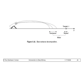
7. Bias-Variance-Noise Decomposition E[ (h(x*) – y*)2 ] = E[ h(x*)2 – 2 h(x*) y* + y*2 ] = E[ h(x*)2 ] – 2 E[ h(x*) ] E[y*] + E[y*2] = E[ (h(x*) – h(x*))2 ] + h(x*)2(lemma) – 2 h(x*) f(x*) + E[ (y* – f(x*))2 ] + f(x*)2(lemma) = E[ (h(x*) – h(x*))2 ] + [variance] (h(x*) – f(x*))2 + [bias2] E[ (y* – f(x*))2 ] [noise]

8. Bias, Variance, and Noise • Variance: E[ (h(x*) – h(x*))2 ] Describes how much h(x*) varies from one training set S to another • Bias: [h(x*) – f(x*)] Describes the average error of h(x*). • Noise: E[ (y* – f(x*))2 ] = E[e2] = s2 Describes how much y* varies from f(x*)

9. 50 fits (20 examples each)

10. Bias

11. Variance

12. Noise

13. 50 fits (20 examples each)

14. Distribution of predictions at x=2.0

15. 50 fits (20 examples each)

16. Distribution of predictions at x=5.0

17. Measuring Bias and Variance • In practice (unlike in theory), we have only ONE training set S. • We can simulate multiple training sets by bootstrap replicates • S’ = {x | x is drawn at random with replacement from S} and |S’| = |S|.

18. Procedure for Measuring Bias and Variance • Construct B bootstrap replicates of S (e.g., B = 200): S1, …, SB • Apply learning algorithm to each replicate Sb to obtain hypothesis hb • Let Tb = S \ Sb be the data points that do not appear in Sb (out of bag points) • Compute predicted value hb(x) for each x in Tb

19. Estimating Bias and Variance (continued) • For each data point x, we will now have the observed corresponding value y and several predictions y1, …, yK. • Compute the average prediction h. • Estimate bias as (h – y) • Estimate variance as Sk (yk – h)2/(K – 1) • Assume noise is 0

20. Approximations in this Procedure • Bootstrap replicates are not real data • We ignore the noise • If we have multiple data points with the same x value, then we can estimate the noise • We can also estimate noise by pooling y values from nearby x values