Download
1 / 25
250 likes | 409 Views
Bayesian Reconstruction of Surface Roughness and Depth Profiles M. Mayer 1 , R. Fischer 1 , S. Lindig 1 , U. von Toussaint 1 , R. Stark 2 , V. Dose 1 1 Max-Planck-Institut für Plasmaphysik, EURATOM Association, Garching, Germany

E N D
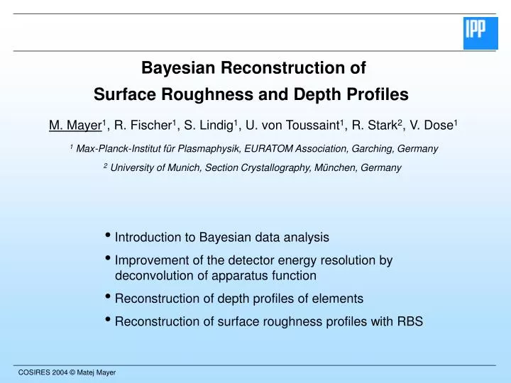
Bayesian Reconstruction of Surface Roughness and Depth Profiles M. Mayer1, R. Fischer1, S. Lindig1, U. von Toussaint1, R. Stark2, V. Dose1 1 Max-Planck-Institut für Plasmaphysik, EURATOM Association, Garching, Germany 2 University of Munich, Section Crystallography, München, Germany • Introduction to Bayesian data analysis • Improvement of the detector energy resolution by deconvolution of apparatus function • Reconstruction of depth profiles of elements • Reconstruction of surface roughness profiles with RBS
MeV Ion Beam Analysis Sample MeV ions E • Elemental composition and depth profiles of elements • Quantitative without reference samples • Overlapof mass- and depth-information • Complicated data analysis • Limited energy resolution of solid state detectors • Limits to mass- and depth resolution
“Classical” IBA Data Analysis Forward calculation Sample p(dq, I) = f(2) Parameters q (layer thickness, layer composition, ...) “Classical” data analysis fitting: 1. Assume sample parameters q 2. Perform forward calculation, calculate 2 3. Vary q until 2is minimal
Bayesian Data Analysis Forward calculation p(dq, I) Sample Parameters q p(qd, I) Backward calculation, inverse problem p(qI): Prior probability I: Additional background information Bayes’ theorem
Bayesian Data Analysis (2) How to choose the prior probabilityp(qI)? Most uninformative prior for spectra is the entropic prior J. Skilling 1991 Solution with maximum information entropy Additional previous information about q can be included Many solutions with identical entropy Select simplest model consistent with the data Adaptive kernels R. Fischer et al., 1996 Favours smooth solutions Marginalization Allows to eliminate uninteresting variables
Bayesian Data Analysis (3) The resulting distribution p(q|d, I) contains the complete knowledge of q mean value, most probable value of q error interval for q Note that 2-minimising(fitting) will find most probable value
< 1 keV straggling < 1 keV 10-15 keV Deconvolution of the Apparatus Function Sample MeV Detector Measured spectrum: A: Apparatus function f(E): Spectrum for “ideal” detector Discrete spectrum: Direct inversion: Does not work in presence of noise
Deconvolution of the Apparatus Function (2) • Example: Mock data set • blurred with Gaussian apparatus function • noise added with Poisson statistics R. Fischer et al., NIM B136-138 (1998) 1140
Deconvolution of the Apparatus Function (3) • Example: Cu on Si • Apparatus function measured with ultra-thin Co layer • Initial resolution: 19 keV FWHM • After deconvolution: 3 keV FWHM • better by factor 3 than theoretical limit of 8 keV for solid state detectors 2.6 MeV 4He, 165° R. Fischer et al., Phys. Rev. E55 (1997) 6667 R. Fischer et al., NIM B136-138 (1998) 1140
Deconvolution of the Apparatus Function (4) • Example: Cu on Si • Error of apparatus function is taken into account • Error bars, confidence intervals are obtained R. Fischer et al., Phys. Rev. E55 (1997) 6667 R. Fischer et al., NIM B136-138 (1998) 1140
Deconvolution of the Apparatus Function (5) • Example: Co-Au multilayer • Apparatus function for Co and Au from ultra-thin films R. Fischer et al., Phys. Rev. E55 (1997) 6667 R. Fischer et al., NIM B136-138 (1998) 1140
Reconstruction of depth profiles D Forward calculation • “Classical” data analysis: • Minimise 2 by varying elemental concentrations in layers • Many parameters (100) simulated annealing • C. Jeynes et al., J. Phys. D: Appl. Phys. 36 (2003) R97 Fast + reliable, sufficient for many applications • But: Not a full solution of the inverse problem • Exactly one result (with 2min) • p(q |d, I) remains unknown no error bars or confidence intervals
Reconstruction of depth profiles (2) D p(q|d, I) • Bayesian data analysis: • Calculate p(q|d, I) using maximum entropy prior • q : Concentrations of elements in the layers
Plasma 12C D 12C before 13C after (scaled) 13C 12C Counts Energy of backscattered 4He [keV] Reconstruction of depth profiles (2) Mixture of 13C/12C due to plasma exposure Depth profiles from Bayesian data analysis U. von Toussaint et al., New Journal of Physics 1 (1999) 11.1
after before Concentration Data Simulation Counts after Concentration Channel Depth [1015 atoms/cm2] Reconstruction of depth profiles (3) 12C 12C 13C O U. von Toussaint et al., New Journal of Physics 1 (1999) 11.1 Note asymmetric confidence intervals
Layer roughness Substrate roughness Distribution p(d) Distribution p(j) Reconstruction of surface roughness distributions In on Si, 2 MeV 4He, 165° Other types of roughness: N. Barradas et al., NIM B217 (2004) 479
L Reconstruction of surface roughness distributions (2) Distribution p(d) ... + + = + M. Mayer, NIM B194 (2002) 177 Correlation effects are neglected valid, if lateral variation L > d for typical RBS angles of 160°-170°
Reconstruction of surface roughness distributions (3) 2 MeV 4He, Ni/Al/O on C 1.5 MeV 4He, Ni on C Distribution p(d)? G-distribution is successful in many cases M. Mayer, NIM B194 (2002) 177 Can we use RBS for measuring p(d) without prior knowledge of the distribution function?
SEM AFM 2 mm 2 mm Reconstruction of surface roughness distributions (4) RBS 2 MeV 4He, 165° Reconstruction of p(d) from RBS 200 nm In on Si
Reconstruction of surface roughness distributions (5) Film thickness distribution RBS spectrum Simulation How well does this compare with other methods?
2 mm Intensity of backscattered electrons depends on In thickness Thickness distribution from grey-values Reconstruction of surface roughness distributions (6) secondary electrons tilt 70° backscattered electrons 25 keV, normal incidence
2 mm Reconstruction of surface roughness distributions (7) • Good agreement for large blobs (around 200 nm) • Small blobs are only visible with RBS and SEM, but not AFM
Disadvantages of Bayesian Data Analysis • Computational: • Complicated (and sometimes scaring) mathematics • Longer computing times, compared to fitting • Experimental: • High quality experimental data required • – apparatus function with good statistics • – reliable energy calibration • – ... • longer experimental time
Conclusions • Bayesian data analysis provides a consistent probabilistic theoryfor the solution of inverse problems • Determines sample parameters plus confidence intervals • Uncertainties of input parameters can be taken into account • Deconvolution of apparatus function: Resolution improvement by factor 6 • Depth profiles of elements with confidence intervals • Surface-roughness distribution from RBS New method for surface roughness measurements