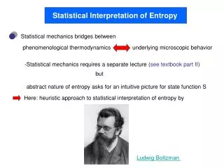
The Statistical Interpretation of Entropy

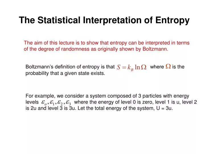
1. The Statistical Interpretation of Entropy The aim of this lecture is to show that entropy can be interpreted in terms of the degree of randomness as originally shown by Boltzmann. Boltzmann’s definition of entropy is that where  is the probability that a given state exists. For example, we consider a system composed of 3 particles with energy levels where the energy of level 0 is zero, level 1 is u, level 2 is 2u and level 3 is 3u. Let the total energy of the system, U = 3u.

2. e3 3u e2 2u e1 u eo 0 a =1 c = 6 b = 3 a; all three particles in level 1; probability of occurrence 1/10 b; one particle in level 3, 2 particles in level 0; 3/10 c; one particle in level 2, 1 particle in level 1, one particle in level 0; 6/10 The total energy of 3u can be present with various configurations or microstate complexions. Distinguishable complexions for U = 3u. All 3 of these complexions or microstates correspond to a single “observable” macrostate.

3. where n particles are distributed among energy levels such that no are in level eo, n1 are in level eo, etc. distribution a; distribution b; distribution c; In general the number of arrangements or complexions within a single distribution is given by

4. The most probable distribution is determined by the set of numbers ni that maximizes. Since for real systems the numbers can be large (consider the number in 1 mole of gas), Stirling’s approximation will be useful, The observable macrostate is determined by constraints. constant energy in the system constant number of particles in the system

5. Any interchange of particles among the energy levels are constrained by the conditions: A B Also using the definition and Stirling’s approximation;

6. Technique of Lagrange multipliers which is a method for finding the extrema of a function of several variables subject to one or more constraints. We will multiply equation A by a quantity b, which has the units of reciprocal energy. D The constraints on the particle numbers impose a condition on , C What we need is to find the most likely microstate or complexion and that will be given by the maximum value of . This occurs when equations A, B and C are simultaneously satisfied.

7. Equation B is multiplied by a dimensionless constant a, E Equations C, D and E are added to give, i.e.,

8. This can only occur is each of the bracketed quantities are identically zero, rearranging for the ni, and summing over all r energy levels,

9. The quantity is very important and occurs very often in the study of statistical mechanics. It is called the partition function, P. Then, This allows us to write the expression for ni in convenient form,

10. So, the distribution of particles maximizing  is one in which the occupancy or population of the energy levels decreases exponentially with increasing energy. We can identify, the undetermined multiplier b using the following argument connecting  with entropy, S. Consider two similar systems a and b in thermal contact with entropies Sa and Sb and associated thermodynamic probabilities aand b. Since entropy (upper case) is an extensive variable, the total entropy of the composite system is

11. The thermodynamic probability of the composite system involves a product of the individual probabilities, Since our aim is to connect  with entropy, S,, we seek Then we must have

12. The only function satisfying this is the logarithm, so that we must have where k is a constant. Now we can identify the quantity b. We start with the condition, C and make the substitution in C for from

13. Expanding rearranging = 0 and solving for b,

14. But we can see that, The constant volume condition results from the fixed number of energy states. The from the combined 1st and 2nd Law and finally

15. Configurational and Thermal Entropy Mixing of red and blue spheres for unmixed state 1, for mixing of red and blue spheres; Then

16. The total entropy will be given by The number of spatial configurations available to 2 closed systems placed in thermal contact is unity. For heat flow down a temperature gradient we only have th changing. Similarly for mixing of particles A and B the only contribution to the entropy change will be S conf if the redistribution of particles does not cause any shift in energy levels, i.e. . This would be the case of ideal mixing since the total energy of the mixed system would be identical to the sum of the energies of the individual systems. This occurs in nature only rarely.