Download
1 / 12
120 likes | 242 Views
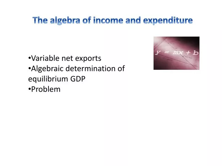
The algebra of income and expenditure. Variable net exports Algebraic determination of equilibrium GDP Problem. Variable net exports. Now we make the more realistic assumption that imports ( M ) depend on the domestic level of income or GDP( Y ).

E N D
The algebra of income and expenditure • Variable net exports • Algebraic determination of equilibrium GDP • Problem
Variable net exports Now we make the more realistic assumption that imports (M) depend on the domestic level of income or GDP(Y). The Marginal Propensity to Import (MPM) is the fraction of the change in income that is spent on imports. That is: Note that:
(a) Variable net export function Net exports = X-M X-M Net exports (trillions of dollars) 0 Real GDP (trillions of dollars) Real GDP (trillions of dollars) 0 6.0 6.0 7.0 7.0 8.0 8.0 9.0 9.0 10.0 10.0 11.0 11.0 12.0 12.0 13.0 13.0 Aggregate expenditure (trillions of dollars) Net exports are added to C, I, and G to yield AE. The addition of net exports: rotates the spending line about the point where net exports are zero (real GDP is $10.0 trillion) C+I+G (b) Aggregate expenditure lines C+I+G+(X-M) Net exports and the aggregate expenditure line
Let AE denote aggregate expenditure . Thus we can say: AE= C + I + G + (X – M) [1] Let NT denote net taxes (taxes minus transfers). Thus we can say: DI = Y – NT The consumption function can be written as: C = a + b(Y – NT) The above and be rewritten as C = a –bNT + bY[2] Where a-bTis autonomous consumption and b is the marginal propensity to consume.
Net exports are described by: X – m(Y – NT) [3] Where m is the marginal propensity to import Now substitute [2] and [3] into [1] to obtain: AE = a – bT + bY + I + G + X – m(Y – NT) In equilibrium AE = Y. Thus Y = a – bT + bY + I + G + X – m(Y – NT) [4] We can rearrange [4] to obtain:
Multiplier Autonomous expenditure AE AE Slope = b - m a-bNT + I + G + X +mNT 0 Y Y*
Problem Let : C= 100 + 0.75(Y – NT) I = 50G = 30 X = 40 M = .15(Y – NT) NT = 100
Let Y denote real GDP. Thus we can say: Y = C + I + G + (X – M) [1] Let NT denote net taxes (taxes minus transfers). Thus we can say: DI = Y – NT. Let NT = $1.0 trillion (net taxes are autonomous).Our consumption function is given by: C = 2.0 + 0.8(Y – NT) = 1.2 + 0.8Y [2] Induced C Autonomous C
AE AE Slope = .75 - .15 = .6 160 0 400 Y
Effects of a change in (autonomous) I Let ΔI = 5 . What is the resulting change in Y?
AE AE’ AE 165 160 0 400 412.5 Y