Download
1 / 62
620 likes | 691 Views
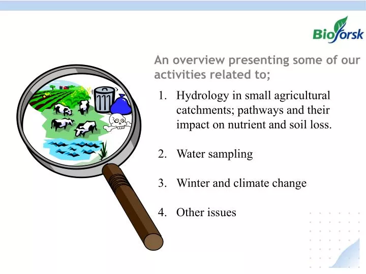
An overview presenting some of our activities related to;. Hydrology in small agricultural catchments; pathways and their impact on nutrient and soil loss. Water sampling Winter and climate change Other issues. Analysis on runoff from agricultural dominated catchment.

E N D
An overview presenting some of our activities related to; Hydrology in small agricultural catchments; pathways and their impact on nutrient and soil loss. Water sampling Winter and climate change Other issues
Analysis on runoff from agricultural dominated catchment • Effects of subsurface drainage systems on hydrology/runoff and nutrient loss • The effect of time resolution on the hydrological characters • The effect of scale on hydrological characters.
Location of catchments Catchment are located in Norway (Mørdre, Skuterud, Høgfoss, Lena), Estonia (Rägina, Räpu) and Latvia (Mellupite) All catchments except Høgfoss and Lena are part of National Agricultural Environmental Monitoring Programmes. Quantifying runoff, nutrient and soil loss
Catchment monitoring calculation of load Discharge measurement using Crump weir, V-notch Water sampling and analysis(TDS, Ntot, Ptot) runoff(mm) N,P,SS loss (kg.ha-1)
http://www.uwsp.edu/cnr/watersheds/GradStudents/Freihoefer.htmhttp://www.uwsp.edu/cnr/watersheds/GradStudents/Freihoefer.htm Flumes H flume http://info1.ma.slu.se/IM/images/RW1.jpg
Point samples strategies. • In general, point sampling routines can be divided into three categories, i.e. • point sampling with variable time intervall • point sampling with fixed time intervall • volume proportional point sampling.
Different ways to calculate load when grab sampling Load(T) = conc(c) x volume in period (V))
Composite volume proportional sampling • An alternative to point sampling systems is volume proportional water samples. • In this case a small water sample is taken each time a preset volume of water has passed the monitoring station. • The sub-samples are collected and stored into one container for subsequent analysis. • This composite sample then represents the average concentration of the runoff water over the sampling period. • A prerequisite is the availability of a head-discharge relation for the location of the measurement station + datalogger
Volume proportional sampling • in which • L total load during sample period • C concentration in composite sample for time period t=1 to t=n • qt hourly discharge at time t • n number of hours represented by the composite sample period
Vannprøvetaking/stofftap • Sampling systems might be combined so as best to suit its purpose. It is assumed that the chemical concentration of runoff water during low flow periods in a way can be considered constant as long as agricultural runoff is concerned. • For low flow periods, a point sampling system with fixed time interval can be implemented, combined with a flow proportional point sampling system for high flow periods.
Vannprøvetaking/stofftap Short-term variability in NO3-N concentrations in Høyjord October 6-9, 1995
Vannprøvetaking/stofftap Phosphorusdynamics in a typicalsmallagriculturalstream(Timebekken, 1.1 km2)
Characteristic for runoff generation is strong seasonality in runoff During growing season very little runoff
Yearly runoff and nutrient loss is generated in only limited number of days An example for the Skuterud catchment, Norway (4.5 km2)
Runoff and nutrient loss in a large catchment Lena catchment (181 km2) Skuterud catchment
Characteristic for many catchments is the large in-day variation in discharge
Flow characteristics of catchments In small Norwegian catchments, yearly discharge shows a high variation, is extremely outlier prone. This is much less pronounced in the large catchments Latvian and Estonian catchments show less variation 1 – specific discharge (l s-1 ha-1); Specific discharge, calculated on average daily and hourly discharge values respectively for Skuterud(4.5 km^2) and Høgfoss(300 km^2)
Winter/snowmelt Winter runoff (Øygarden, 2000) January 30 Runoff: 25 mm Soil loss: 2 kg ha-1 January 31 Runoff: 77 mm Soil loss: 3 050 kg ha-1
Runoff generation caused by freeze/thaw cycles in combination with snowmelt/precipitation
Variation in discharge can be expressed through a flashiness index, showing the rate of change Which factors influence runoff generation? hour (in- day variation); day;
Runoff generation, scale and subsurface drainage Subs dr. Subs dr. Subs dr. The size of the catchment is important and share of agr. land. Subsurface drainage systems seem to have a significant influence on runoff generation
drain The effects of subsurface drainage and nutrient – and soil loss groundwater level Drain spacing, L = 8 – 10 m Drain depth, d = 0.8 – 1.0 m bss.
Soil types important Macropore/preferential flow Fast transport to subsurface drainage systems Transporting soil particles/phosphorus?
Base flow index Qt – total runoff Qd – direct runoff • Has been calculated using the smooth minima technique (Gustard et al, 1992) • Input average daily discharge values • No programs available to calculate on hourly discharge values • Digital filter is looked at (Chapman, Eckhard).
Some conclusions and challenge • Norwegian small agricultural catchments show higher variation in discharge compared to those in Estonian and Latvia • Factors playing a role seem to be • Subsurface drainage systems • The size of catchment • Share of the agricultural land • Time resolution seems to play an important role, small catchment -> high resolution data important • Challenge to calculate baseflow on hourly values • Only when we have models which simulate the dominating flow generating processes and there affect on nutrient and soil loss under our prevailing climatic conditions we can be successful in implementing the WFD
Do we have models to deal with those situations • Several models are testet in a Norwegian catchment • SWAT (water balance, nutrient and soil loss) • The SWAT model has also been applied in Norway as part of EuroHarp and Striver, two EU – projects (large scale) • The model is tested now in Skuterud • DRAINMOD, developed at NCSU (Skaggs) simulating subsurface drainage/surface runoff/nitrogen dynamics • HBV – model (hydrology) • INCA – model (hydrology, nutrient dynamics) • SOIL/SOIL_NO and COUP (hydrology,nitrogen); have been tested (developed by SLU) • WEPP (Water erosion prediction model) tested on small plots
IS ice too cold for non – Scandinavian models • Johannes Deelstra and Sigrun H. Kværnø • Based partly on a presentation we had focussing on the winter season and nutrient and soil loss during that period, results of EuroHarp project (EU)
What is so special with a winter • The winter is the coldest season of the year and for most meteorological purposes is taken to include December, January, and February in the Northern Hemisphere. • Air temperatures below 0 oC • Precipitation as snow • Water turns into ice • Slippery roads, traffic problems, accidents
Characteristics of Nordic winter • Winter season - the time period between the first and last day with an average daily temperature below zero. • Often characterised by several freeze/thaw cycles
liquid water content TDR equipment Neutron scattering total water content Infiltration and frozen soils, is there any, and how to measure • Skuterud catchment 2001/2002
Infiltration and frozen soils, is there any, and how to measure • Skuterud catchment 2001/2002
Infiltration and frozen soils, is there any and how to measure • Infiltration tests in frozen soils, Vandsemb catchment (2002) Excavation in May 2002
Infiltration and frozen soils, is there any and how to measure • Infiltration tests in frozen soils, Vandsemb catchment (2002)
Infiltration and frozen soils ―>latent heat of freezing • Water, when freezing releases heat, latent heat of freezing. • This know property is used in frost protection • The effects of not including the latent heat of freezing in the simulation leads to errors in simulated frost depth.
The effect of latent heat on soil frost development Season 2000 - 2001 Season 2002 - 2003
The effect of snow on soil frost development Season 2000 - 2001 Season 2002 - 2003
The effects of freeze/thaw cycles on aggregate stability • Reduction: • Clay: 25 % after 6 cycles • Silt: 50 % after 1 cycle more frequent alterations between mild and cold periods can be expected to increase the erosion risk erosion risk is higher on silt than on clay
The effects of freeze/thaw cycles on shear strength • Reduction: 25 % after 6 cycles Erosion risk increases under unstable winter conditions Wet soils particularly vulnerable