Download
1 / 21
230 likes | 403 Views
Comparison of Estimation Methods of Structural Models of Credit Risk. Jeff Blokker, Shafigh Mehraeen, Won Chase Kim, Bobak Javid, and John Weng. MS&E 347 Term Project Stanford University June 2009. Structural Models.

E N D
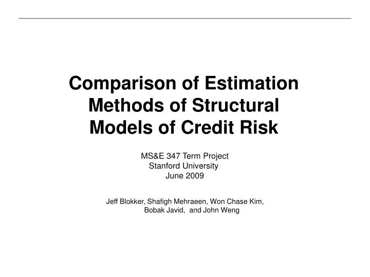
Comparison of Estimation Methods of Structural Models of Credit Risk Jeff Blokker, Shafigh Mehraeen, Won Chase Kim, Bobak Javid, and John Weng MS&E 347 Term Project Stanford University June 2009
Structural Models • Structural models refer to models that look at the evolution of the capital structure of the firm to evaluate their credit risk. • Merton’s model (1974) was the first modern credit risk model that was considered a structural model. • It assumes the capital structure of the firm is composed of equity St and a zero coupon bond of value Dt with face value F. • Then the asset value of the firm is the sum of the equity and debt. • Assumptions • No transaction costs, no bankruptcy costs, no taxes, • infinite divisibility of assets, unrestricted borrowing and lending, • constant interest rate • GBM of firm’s asset value.
Merton’s Model • If the value of the firm at the maturity date T is less than K then the firmwill be unable to repay the debt. • The payoff structure at T is:
Merton’s Model • The firm’s equity St represents a European call option on the firm’s assets with maturity T. • The Bond represents a risk free loan F with maturity T plus selling a European put option with strike F and maturity T • Merton’s model assumes that the firm can only default at time T. • The value of the firm is assumed to follow the SDE • With the volatility of the firm’s asset value, a constant interest rate r, and risk neutral Brownian motion
Merton’s Model • Applying the Black Scholes equation to the equity value of the firm yields • To implement Merton’s model we need an estimate of : • Volatility of the asset value - • Drift of the asset value -
First Passage Model • The first passage model is an extension of the Merton model • Default at any time T1 < T if the asset value Vt crosses the barrier K.
First Passage Model • At T the value of the equity is • This is a Down and Out call option with formula when F>=K when F<K
Model Calibration • To implement the first passage model we need an estimate of • Asset volatility - • Default barrier - K • Drift - • We compare three methods for calibration: • Inversion Method • MLE • Iterative Method - KMV
Inversion Method • for Merton’s model • for First Passage model • From Ito’s formula we get • Comparing coefficients of the two SDE equations we conclude that where f is a simple call option (Merton) or down-and-out call option (First Passage model)
Maximum Likelihood Estimate (MLE) • Proposed by Duan (1994) • Given a time sequence of equity values , we can estimate a time sequence of asset values , volatility , drift , and the barrier K. • We denote the probability density function for the equity value at ti given the equity value at ti-1 and the parameter vector . • Then the log-likelihood is given by • Using the previously defined function and assuming it is differentiable and invertible we can write where is the P-density of Vt given Vt-1.
Maximum Likelihood Estimate (MLE) • MLE for the Merton’s Model • Letting be the time between observations where
Maximum Likelihood Estimate (MLE) • MLE for the First Passage Model
Iteration Method - KVM • Estimation of and • Asset values Vt are implied from equity value • Returns and • Volatility • Drift • Repeat until convergence. • Equivalent to EM algorithm and asymptotically converges to ML • For the Merton’s model, much faster than ML • For the First Passage model, no analytical formula.
Monte Carlo Simulation Environment • Asset value paths are generated by GBM with constant parameters • V0=1.5 • F = 1.0 • K/F = 0.8 or 1.2 • T = 2 • volatility = 0.3 • Drift = 0.1 • R = 5% • 2500 samples generated and down-sampled to 250 per year • To reduce bias (In reality, we only observe daily equity values) • Only keep the value process which does not default • Converted to equity value paths by BS formula (call or DOC) • Use equity paths in each model to recover parameters
Results – Merton Model Volatility Drift
Results –First Passage Model F>=K Drift Volatility Default Barrier
Results –First Passage Model F<K Volatility Default Barrier Drift
Empirical analysis: an example • From the model we can calculate corporate default probability
Conclusion • Three estimation methods are compared for two structural credit models • For Merton’s model, ML and KMV are equivalent and superior to inversion • For the first passage model, ML is the only option but estimation of barrier is not an easy problem. • Drift estimation is also difficult but it is out of our interest • When K/F is small, two models does not make much difference • Further research must be done for benefits of the first passage model • Results from this projects can be extended for various applications • Default probability estimation • Term structure of credit spread