3.3 Network-Centric Community Detection

1. 3.3 Network-Centric Community Detection • A Unified Process

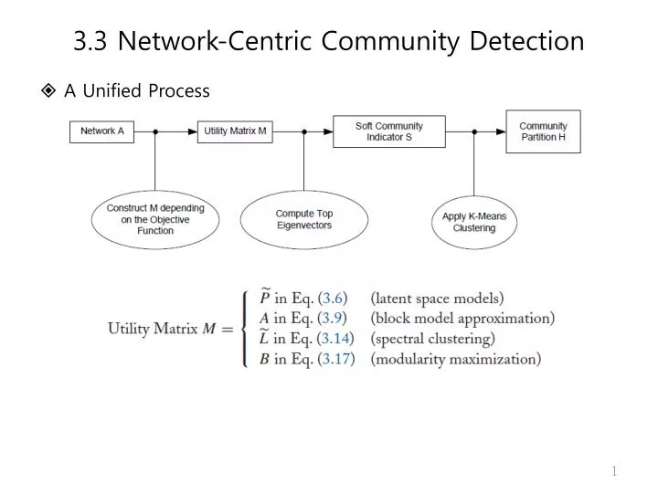
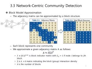
2. 3.3 Network-Centric Community Detection • Comparison • Spectral clustering essentially tries to minimize the number of edges between groups. • Modularity consider the number of edges which is smaller than expected. • The spectral partitioning is forced to split the network into approximately equal-size clusters.

3. 3.4 Hierarchy-Centric Community Detection • Hierarchy-centric methods • build a hierarchical structure of communities based on network topology • two types of hierarchical clustering • Divisive • Agglomerative • Divisive Clustering • 1. Put all objects in one cluster • 2. Repeat until all clusters are singletons • a) choose a cluster to split • what criterion? • b) replace the chosen cluster with the sub-clusters • split into how many?

4. 3.4 Hierarchy-Centric Community Detection • Divisive Clustering • A Method: Cut the “weakest” tie • At each iteration, find out the weakest edge. • This kind of edge is most likely to be a tie connecting two communities. • Remove the edge. • Once a network is decomposed into two connected components, each component is considered a community. • Update the strength of links. • This iterative process is applied to each community to find sub-communities.

5. 3.4 Hierarchy-Centric Community Detection • Divisive Clustering • “Finding and evaluating community structure in networks,” M. Newman and M. Girvan, Physical Review, 2004 • find the weak ties based on “edge betweenness” • Edge betweenness • the number of shortest paths between pair of nodes pass along the edge • utilized to find the “weakest” tie for hierarchical clustering • where • is the total number of shortest paths between nodes and • is the number of shortest paths between nodes and that pass along the edge .

6. 3.4 Hierarchy-Centric Community Detection • Divisive Clustering • The edge with higher betweennesstends to be the bridge between two communities • It is used to progressively remove the edges with the highest betweenness.

7. 3.4 Hierarchy-Centric Community Detection • Divisive Clustering • “Finding and evaluating community structure in networks,” M. Newman and M. Girvan, Physical Review, 2004 • Example • Negatives for divisive clustering • edge betweenness-based scheme requires high computation • One removal of an edge will lead to the recomputation of betweenness for all edges

8. 3.4 Hierarchy-Centric Community Detection • Agglomerative Clustering • begins with base (singleton) communities • merges them into larger communities with certain criterion. • One example criterion: modularity • Let be the fraction of edges in the network that connect nodes in community to those in community • Let , then the modularity • values approaching indicate networks with strong community structure • values for real networks typically fall in the range from 0.3 to 0.7 동일한 Community 안의 Edge 수 – 서로 다른 Community 들 간의 Edge수

9. 3.4 Hierarchy-Centric Community Detection • Agglomerative Clustering • Two communities are merged if the merge results in the largest increase of overall modularity • The merge continues until no merge can be found to improve the modularity. Dendrogram according to Agglomerative Clustering based on Modularity

10. 3.4 Hierarchy-Centric Community Detection • Agglomerative Clustering • In the dendrogram, the circles at the bottom represent the individual nodes of the network. • As we move up the tree, the nodes join together to form larger and larger communities, as indicated by the lines, until we reach the top, where all are joined together in a single community. • Alternatively, the dendrogram depicts an initially connected network splitting into smaller and smaller communities as we go from top to bottom. • A cross section of the tree at any level, such the one indicated by a dotted line, will give the communities at that level.

11. 3.4 Hierarchy-Centric Community Detection • Divisive vs. Agglomerative Clustering • Zachary's karate club study Zachary observed 34 members of a karate club over a period of two years. During the course of the study, a disagreement developed between the administrator (34) of the club and the club's instructor (1), which ultimately resulted in the instructor's leaving and starting a new club, taking about a half of the original club's members with him

12. 3.4 Hierarchy-Centric Community Detection • Divisive vs. Agglomerative Clustering • Divisive • “Community structure in social and biological networks”, Michelle Girvan, and M. E. J. Newman, 2001  Using edge-betweeness • Agglomerative • “Fast algorithm for detecting community structure in networks”, M. E. J. Newman, 2003  Using modularity Agglomerative Divisive

13. Summary of Community Detection • Node-Centric Community Detection • cliques, k-cliques, k-clubs • Group-Centric Community Detection • quasi-cliques • Network-Centric Community Detection • Clustering based on vertex similarity • Latent space models, block models, spectral clustering, modularity maximization • Hierarchy-Centric Community Detection • Divisive clustering • Agglomerative clustering

14. 3.5 Community Evaluation • Here, we consider a “Social Network with Ground Truth” • Community membership for each actor is known  an ideal case • For example, • A synthetic networks generated based on predefined community structures • L. Tang and H. Liu. “Graph mining applications to social network analysis.” In C. Aggarwaland H.Wang, editors, Managing and MiningGraph Data, chapter 16, pages 487.513.Springer, 2010b • Some well-studied tiny networks like Zachary’s karate club with 34 members • M.Newman. “Modularity and community structure in networks.” PNAS, 103(23):8577.8582, 2006a. • Simple comparison between the ground truth with the identified community structure • Visualization • One-to-one mapping

15. 3.5 Community Evaluation • The number of communities after grouping can be different from the ground truth • No clear community correspondence between clustering result and the ground truth • Normalized Mutual Information (NMI) can be used How to measure the clustering quality? Each number denotes a node, and each circle or block denotes a community  1) Both communities {1, 3} and {2} map to the community {1, 2, 3} in the ground truth 2) The node 2 is wrongly assigned

16. 3.5 Community Evaluation • Entropy • 확률변수의 불확실성을 측정하기 위한 것 • Measure of disorder • The information volume contained in a random variable X (or in a distribution X) • X의 엔트로피는 X의 모든 가능한 결과값 x에 대해 x의 발생 확률과 그 확률의 역수의 로그 값의 곱의 합 • 일반적으로 지수 b의 값으로서 2나 오일러의 수 e, 또는 10이 많이 사용된다. b=2인 경우에는 엔트로피의 단위가 비트(bit)이며, b=e이면네트(nat), 그리고 b=10인 경우에는 디짓(digit)이 된다.

17. 3.5 Community Evaluation • Entropy와 동전 던지기 [fromwikipedia] • 앞면과 뒷면이 나올 확률이 같은 동전을 던졌을 경우의 엔트로피를 생각해 보자. 이는 H,T 두 가지의 경우만을 나타내므로 엔트로피는 1이다. • + )=1 • 한편 공정하지 않는 동전의 경우에는 특정 면이 나올 확률이 상대적으로 더 높기 때문에 엔트로피는 1보다 작아진다. 우리가 예측해서 맞출 수 있는 확률이 더 높아졌기 때문에 정보의 양, 즉 엔트로피는 더 작아진 것이다. 동전던지기의 경우에는 앞,뒤 면이 나올 확률이 1/2로 같은 동전이 엔트로피가 가장 크다. • 엔트로피를 불확실성(uncertainity)과 같은 개념이라고 인식할 수 있다. • 불확실성이 높아질수록 정보의 양은 더 많아지고 엔트로피는 더 커진다.

18. 3.5 Community Evaluation • Mutual Information (상호 정보량) • It measures the shared information volume between two random variables (or two distributions) • 두 확률 변수 (또는두 분포)X, Y가 얼마나 밀접한 관계가 있는지 또는 얼마나 서로간에 의존을 하는지를 측정 • 국문 참고 문헌 • http://shineware.tistory.com/7 • http://www.dbpia.co.kr/Journal/ArticleDetail/339089

19. 3.5 Community Evaluation • Normalized Mutual Information (NMI, 정규화된 상호 정보량) • It measures the shared information volume between two random variables (or two distributions) • 두 확률 변수 (또는 두 분포) X, Y가 얼마나 밀접한 관계가 있는지를 측정 • The values is between 0 and 1 • Consider a partition as a random variable, we can compute the matching quality between ground truth and the identified clustering

20. 3.5 Community Evaluation • NMI Example (1/2) • Partition a (): [1, 1, 1, 2, 2, 2] • Partition b (): [1, 2, 1, 3, 3, 3] 1, 2, 3 4, 5, 6 1, 3 2 4, 5,6

21. 3.5 Community Evaluation • NMI Example (2/2) • Partition a (): [1, 1, 1, 2, 2, 2] • Partition b (): [1, 2, 1, 3, 3, 3] 1, 2, 3 4, 5, 6 1, 3 2 4, 5,6 =0.8278

22. 3.5 Community Evaluation • Accuracy of Pairwise Community Memberships • Consider all the possible pairs of nodes and check whether they reside in the same community • An error occurs if • Two nodes belonging to the same community are assigned to different communities after clustering • Two nodes belonging to different communities are assigned to the same community • Construct a contingency table

23. 3.5 Community Evaluation • Accuracy of Pairwise Community Memberships 1, 2, 3 4, 5, 6 1, 3 2 4, 5, 6 Ground Truth Clustering Result Accuracy = (4+9)/ (4+2+9+0) = 0.86

24. 3.5 Community Evaluation • Accuracy of Pairwise Community Memberships • Balanced Accuracy (BAC) = 1 – Balanced Error Rate (BER) • This measure assigns equal importance to “false positives” and “false negatives”, so that trivial or random predictions incur an error of 0.5 on average.

25. 3.5 Community Evaluation • Accuracy of Pairwise Community Memberships • Balanced Accuracy (BAC) = 1 – Balanced Error Rate (BER) 0.83

26. 3.5 Community Evaluation • Evaluation without Ground Truth • This is the most common situation • Quantitative evaluation functions: modularity • Once we have a network partition, we can compute its modularity • The method with higher modularity wins • modularity • Let be the fraction of edges in the network that connect nodes in community to those in community • Let , then the modularity • values approaching indicate networks with strong community structure • values for real networks typically fall in the range from 0.3 to 0.7 동일한 Community 안의 Edge 수 – 서로 다른 Community 들 간의 Edge수

27. Book Available at Morgan & claypool Publishers Amazon If you have any comments,please feel free to contact: • Lei Tang, Yahoo! Labs, ltang@yahoo-inc.com • Huan Liu, ASU huanliu@asu.edu