Download
1 / 26
260 likes | 425 Views
Linking land cover change to pressures on biodiversity. http://www.creaf.uab.es/biopress/. Question: How have past changes in land cover affected Biodiversity ? Why: Legislative imperative to protect the environment. EEA is our key stakeholder How: Measuring land cover change by

E N D
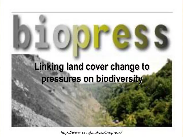
Linking land cover change to pressures on biodiversity http://www.creaf.uab.es/biopress/
Question: • How have past changes in land cover affected Biodiversity ? • Why: • Legislative imperative to protect the environment. EEA is our key stakeholder • How: • Measuring land cover change by manual interpretation of aerial photos • Pressure – State – Impact Funded by EC – Framework 5: Project coordinator: Dr. France Gerard ffg@ceh.ac.uk Tel: +44(0)1487 773381 Centre for Ecology and Hydrology Monks Wood, Abbots Ripton PE28 2 LS, UK http://www.creaf.uab.es/biopress/
Phase I 1950 Aerial photos 1990 CORINE LC Aerial photos EO 2000 CORINE LC Aerial photos 2000+ EO To Land cover Conversion matrix From • Region Specific Pressures • Abandonment • Intensification • etc… Human Population Census Statistics on agriculture Transport Data Etc… Cause & Effect Stratification & Extrapolation Zone Semi quantitative Pressure – state model Biodiversity Phase II Pressures
Key steps – land cover change (1950 – 2000) Stratification strategy Interpreters rules: 2 manuals Windows: CORINE Land Cover backdating Transects: photo to photo interpretation Sampling sitesacross Europe: 100 windows, 50 transects Location, acquisition, pre-processing of aerial photography Windows: 1950 Transects: 1950, 1990, 2000 Workshop: Training of interpreters CORINE backdating: Change matrices (1950-1990) Transect interpretation: Change matrices (1950,1990,2000) Quality assessment for pilot sites Assessment of results by external experts Extrapolating the matrices to produce a European land cover change product
Key steps – Pressure-State-Impact Improve pressure - state model Integrating with non RS data to quantify pressures and assessment of impact on biodiversity Spatial framework for integration, extrapolation & reporting RS of landscape features for quantifying pressures Land Cover Change data Error Propagation
Sample of Natura2000 Sites Stratification: Biogeographical Regions Map of Europe (BRME) 75 Windows: 30 x 30 km (black) 59 Transects: 2 x 15 km (red) Focussing on 4 Annex-I habitats which are found in main bio-geographical regions: (i) Freshwater habitats, (ii) Natural and semi-natural grassland formations, (iii) Raised bogs and mires and fens and (iv) Forests.
Sampling Area Distribution of window area with respect to biogeographic regions as defined by the Biogeographic Regions Map of Europe (BRME)
Sampling Area Area proportion of Europe calculated from the Biogeographic Regions Map of Europe (BRME)
Change matrices for ~100 Natura2000 sites Backdating CORINE 1990 with aerial photos of the 1950’ies 30 km x 30 km windows = total of 90,000 km2
Backdating CORINE land cover 1990 to 1950’ies 30x30kmwindowscentred on Natura2000 site CORINE LC 1990 CORINE LC’90 on aerial photos of 1950’ies Area around Zaventem airport, Brussels, Belgium
Semi natural shrub & woodlands Photo to Photo Interpretation 15 x 2 km transects from least intensive to most intensive Catalonia, Spain 1990 1950 Town
1998 Catalonia, Spain 1956
Marianskolazenske hadce (1659ha) 132 Dumps 131 Minerals 112 Built 231 Pasture 243 Ag’ mosaic 242 Ag’Complex 211 Arable 313 Mixed 322 Moors 324 Transitional Fluxes > 100ha Fluxes > 1000ha Fluxes > 5000ha 312 Coniferous Change 1990 1950 Window 185 Czech Republic
Poelbos-Marais de Jette (90ha) Valleigebied tussen Melsbroek... (1445ha) Zoniënwoud (2761ha) Change 1990 1950 Window 210 Belgium 242 Ag’complex 231 Pasture 243 Ag’mosaic 311 Brd wood 313 Mxd wood 142 Sports 124 Airport 112 Urban 121 Industrial Fluxes > 100ha Fluxes > 1000ha Fluxes > 5000ha 324 Scrub 211 Arable
Germany Transect - De1 All transect and window data are stored in a common database
Germany Transect – De8 All transect and window data are stored in a common database
The Netherlands: Arable into harbour & build-up: Urbanisation
Finland: Peatbogs into arable land: Intensification
Germany: First intensification then abandonment 2000 1990 1950
U U U U U U U U U U U U U U U U U U U U U U U U U U U U U U U U 1.3.3. Construction sites U U U U U U U U U U U U U U U U U U U 1.4.1. Green urban areas U U U U U U U U U U U U U U U U U U U 1.4.2. Sport and leisure facilities U U U U U U U U U U U I I I I I I I 2.1.1. Non-irrigated arable land U U U U U U U U U U U I I I I I I I 2.1.2. Permanently irrigated land U U U U U U U U U U U Dr Dr Dr Dr Dr Dr Dr I 2.1.3. Rice fields U U U U U U U U U U U I I I I I 2.2.1. Vineyards U U U U U U U U U U U I I I I I I 2.2.2. Fruit trees and berry plantations U U U U U U U U U U U I I I I I I I I 2.2.3. Olive groves U U U U U U U U U U U I I I I I I I I 2.3.1. Pastures U U U U U U U U U U U I I I I I I I I 2.4.1 Annual crops associated with permanent crops U U U U U U U U U U U I I I I I 2.4.2. Complex cultivation patterns U U U U U U U U U U U I I I I I I I I 2.4.3. Land principally occupied by agriculture, with significant areas of natural vegetation U U U U U U U U U U U I I I I I I D I 2.4.4. Agro-forestry areas U U U U U U D D U U U I I I I I I I I I I 3.1.1. Broad-leaved forests U U U U U U D D U U U I I I I I I I I I I 3.1.2. Coniferous forests U U U U U U D D U U U I I I I I I I I I I 3.1.3. Mixed forests U U U U U U U U U U U I I I I I I I I I I 3.2.1. Natural grasslands U U U U U U U U U U U I I I I I I I I I I 3.2.2. Moors and heathland U U U U U U U U U U U I I I I I I I I I I 3.2.3. Sclerophyllous vegetation U U U U U U U U U U U I I I I I I I I I I 3.2.4. Transitional woodland-scrub U U U U U U U U U U U I I I I I I I I I 3.3.1. Beaches, dunes, sands U U U U U U U U U U U I I I I I I I I 3.3.2. Bare rocks U U U U U U U U U U U I I I I I I I I I I 3.3.3. Sparsely vegetated areas U U U U U U U U U U U I I I I I I I I I I 3.3.4. Burnt areas U U U U U U U U 3.3.5. Glaciers and perpetual snow U U U U U U U U U U U I I I I I I Dr I I I 4.1.1. Inland marshes U U U U U U U U U U U I I I I I I Dr I I I 4.1.2. Peat bogs U U U U U U U U U U U I I I I I I Dr I I I 4.2.1. Salt marshes U U U U U U U U U U U I I I I I I Dr I I I 4.2.2. Salines U U U U U U U U U U U I I I I I I Dr I I I 4.2.3. Intertidal flats U U U U U U U U U U U I I I I I I Dr I I I 5.1.1. Water courses U U U U U U U U U U U I I I I I I Dr I I I 5.1.2. Water bodies U U U U U U U U U U U I I I I I I Dr I I I 5.2.1. Coastal lagoons U U U U U U U U U U U I I I I I I Dr I I I 5.2.2. Estuaries U U U U U U U U U U U I I I I I I Dr I I I 5.2.3. Sea and oceans U U U U U U U U U U U I I I I I I 6.2.1. Farmed land U U U U U U U U U U U I I I I I I 6.2.2. Plantations (food crops) 6.3.1. Forests U U U U U U D D D U Land cover to pressure conversion TO\T1 1.1.1. 1.1.2. 1.2.1. 1.2.2. 1.2.3. 1.2.4. 1.3.1. 1.3.2. 1.3.3. 1.4.1. 1.4.2. 2.1.1. 2.1.2. 2.1.3. 2.2.1. 2.2.2. 2.2.3. 2.3.1. 2.4.1 2.4.2. 2.4.3. U U U U U U U U U U U U 1.1.1. Continuous urban fabric U U U U U U U U U U U U U U U 1.1.2. Discontinuous urban fabric U U U U U U U U U U U U 1.2.1. Industrial or commercial units U U U U U U U U U U U U U U U 1.2.2. Road and rail networks and associated land U U U U U U U U U U U U U 1.2.3. Port areas U U U U U U U U U U U U U U U 1.2.4. Airports U U U U U U U U U U U U U U U U U 1.3.1. Mineral extraction sites U 1.3.2. Dump sites U I I I I I I I I I I U U U U U U U U U U U I I I I I I I I 6.3.2. Grasslands Priority rules Combination of more than one intensification OR relaxation per case The less natural the process, the more priority (Urbanisation > Intensification > Drainage > Deforestation > Abandonment > Afforestation) in intensification. The less natural the process, the less priority (Urbanisation < Intensification < Drainage < Deforestation < Abandonment < Afforestation) in relaxation
DRIVING FORCES Demographic trends Transport network Urban sprawl Economic pressures Urban sprawl Agricultural policies Economic trends Subsidies Economic trends PRESSURES Urbanisation Deforestation Afforestation Intensification STATE Land Cover Changes Increase in artificial surfaces increase of major roads Forest and transitional woodlands turn into artificial surfaces Forest turned into transitional woodland agricultural areas tuned into forest decrease of arable land and pastures afforestation--intensification IMPACT Impact on Biodiversity Forest fragmentation loss a valuable habitat urban sprawl takes over agricultural land and forest Forest area that turn into urban- forest loss clearcuts- loss of valuable forest habitats Lake-and riverside fields with scattered farmhouses turned into managed forest Loss of valuable open habitat types and ecotones Increase of pine forest with no biodiversity value DPSIR - frameworkFinland - Riihimäki - Hyvinkää
Pressures: How can indicators quantify them ? Why is it so difficult to select indicators? • PRESSURES • Urbanisation • Deforestation • Afforestation • Land Abandonment • Intensification • Drainage • INDICATORS: • Spatial Configuration • Semantic Composition • Temporal Distribution
BIOPRESS’s strategy: • Select indicators that can be used in the short term (even when imperfect) • Identify indicators by pressure, but also by spatial configuration, semantic composition, and temporal distribution. • Weighting indicators using a space-time assessment Priority, ranking, or value of indicators • Bottom-up approach & use of analytical zoning • Suitable spatial scales to tackle habitat information range from 1:5,000 to 1:100,000 and landscape maps are required as input to compute indicators with a spatial component. • Suitable temporal scales are not that clear yet.
2000+ EO • Region Specific Pressures • Abandonment • Intensification • etc… Phase I 1950 Aerial photos 1990 CORINE LC Aerial photos EO 2000 CORINE LC Aerial photos To Land cover Conversion matrix From Integration Human Population Census Statistics on agriculture Transport Data Etc… Socio economic Indicators Cause & Effect Stratification & Extrapolation Zone Semi quantitative Pressure – state model Biodiversity Phase II Pressures

![A [simple] land cover change intercomparison](https://cdn2.slideserve.com/3941152/a-simple-land-cover-change-intercomparison-dt.jpg)