Download
1 / 47
520 likes | 1.3k Views
Fractional fourier transform. Presenter: Hong Wen-Chih. Outline. Introduction Definition of fractional fourier transform Linear canonical transform Implementation of FRFT/LCT The Direct Computation DFT-like Method Chirp Convolution Method Discrete fractional fourier transform

E N D
Fractional fourier transform Presenter: Hong Wen-Chih
Outline • Introduction • Definition of fractional fourier transform • Linear canonical transform • Implementation of FRFT/LCT • The Direct Computation • DFT-like Method • Chirp Convolution Method • Discrete fractional fourier transform • Conclusion and future work
Introduction • Definition of fourier transform: • Definition of inverse fourier transform:
Introduction In time-frequency representation • Fourier transform: rotation π/2+2k π • Inverse fourier transform: rotation -π/2+2k π • Parity operator: rotation –π+2k π • Identity operator: rotation 2k π And what if angle is not multiple of π/2 ?
Introduction . Time-frequency plane and a set of coordinates rotated by angle α relative to the original coordinates
Fractional Fourier Transform • Generalization of FT • use to represent FRFT • The properties of FRFT: • Zero rotation: • Consistency with Fourier transform: • Additivity of rotations: • 2π rotation: Note: do four times FT will equal to do nothing
Fractional Fourier Transform • Definition: • Note: when α is multiple of π, FRFTs degenerate into parity and identity operator
Linear Canonical Transform • Generalization of FRFT • Definition: when b≠0 when b=0 • a constraint: must be satisfied.
Linear Canonical Transform • Additivity property: where • Reversibility property: where
Linear Canonical Transform • Special cases of LCT: • {a, b, c, d} = {0, 1, 1, 0}: • {a, b, c, d} = {0, 1, 1, 0}: • {a, b, c, d} = {cos, sin, sin, cos}: • {a, b, c, d} = {1, z/2, 0, 1}: LCT becomes the 1-D Fresnel transform • {a, b, c, d} = {1, 0, , 1} : LCT becomes the chirp multiplication operation • {a, b, c, d} = {, 0, 0, 1}: LCT becomes the scaling operation.
Implementation of FRFT/LCT • Conventional Fourier transform • Clear physical meaning • fast algorithm (FFT) • Complexity : (N/2)log2N • LCT and FRFT • The Direct Computation • DFT-like Method • Chirp Convolution Method
Implementation of FRFT/LCT • The Direct Computation • directly sample input and output
Implementation of FRFT/LCT • The Direct Computation • Easy to design • No constraint expect for • Drawbacks • lose many of the important properties • not be unitary • no additivity • Not be reversible • lack of closed form properties • applications are very limited
Implementation of FRFT/LCT • Chirp Convolution Method • Sample input and output as and
Implementation of FRFT/LCT • Chirp Convolution Method • implement by • 2 chirp multiplications • 1 chirp convolution • complexity • 2P (required for 2 chirp multiplications) + Plog2P(required for 2 DFTs) Plog2P(P = 2M+1 = the number of sampling points) • Note: 1 chirp convolution needs to 2DFTs
Implementation of FRFT/LCT • DFT-like Method • constraint on the product of t and u (chirp multi.) (FT) (scaling) (chirp multi.)
Implementation of FRFT/LCT • DFT-like Method • Chirp multiplication: • Scaling: • Fourier transform: • Chirp multiplication:
Implementation of FRFT/LCT • DFT-like Method • For 3rd step • Sample the input t and output u as pt and qu
Implementation of FRFT/LCT • DFT-like Method • Complexity • 2 M-points multiplication operations • 1 DFT • 2P (two multiplication operations) + (P/2)log2P(one DFT) (P/2)log2P
Implementation of FRFT/LCT • Compare • Complexity • Chirp convolution method:Plog2P (2-DFT) • DFT-like Method: (P/2)log2P (1-DFT) • DFT: (P/2)log2P (1-DFT) • trade-off: • chirp. Method: sampling interval is FREE to choice • DFT-like method:some constraint for the sampling intervals
Discrete fractional fourier transform • Direct form of DFRFT • Improved sampling type DFRFT • Linear combination type DFRFT • Eigenvectors decomposition type DFRFT • Group theory type DFRFT • Impulse train type DFRFT • Closed form DFRFT
Discrete fractional fourier transform • Direct form of DFRFT • simplest way • sampling the continuous FRFT and computing it directly
Discrete fractional fourier transform • Improved sampling type DFRFT • By Ozaktas, Arikan • Sample the continuous FRFT properly • Similar to the continuous case • Fast algorithm • Kernel will not be orthogonal and additive • Many constraints
Discrete fractional fourier transform • Linear combination type DFRFT • By Santhanam, McClellan • Four bases: • DFT • IDFT • Identity • Time reverse
Discrete fractional fourier transform • Linear combination type DFRFT • transform matrix is orthogonal • additivity property • reversibility property • very similar to the conventional DFT or the identity operation • lose the important characteristic of ‘fractionalization’
Discrete fractional fourier transform • Linear combination type DFRFT • DFRFT of the rectangle window function for various angles : • (top left) α= 0:01, • (top right) α = 0:05, • (middle left) α = 0:2, • (middle right) α = 0:4, • (bottom left) α =π/4, • (bottom right) α =π/2.
(a) = 0.01 • (b) = 0.05 • (c) = 0.2 • (d) = 0.4 • (e) = π/4 • (f) = π/2
Discrete fractional fourier transform • Eigenvectors decomposition type DFRFT • DFT : F=Fr – j Fi • Search eigenvectors set for N-points DFT
Discrete fractional fourier transform • Eigenvectors decomposition type DFRFT • Good in removing chirp noise • By Pei, Tseng, Yeh, Shyu • cf. : DRHT can be
Discrete fractional fourier transform • Eigenvectors decomposition type DFRFT • DFRFT of the rectangle window function for various angles : • (top left) α= 0:01, • (top right) α = 0:05, • (middle left) α = 0:2, • (middle right) α = 0:4, • (bottom left) α =π/4, • (bottom right) α =π/2
Discrete fractional fourier transform • Group theory type DFRFT • By Richman, Parks • Multiplication of DFT and the periodic chirps • Rotation property on the Wigner distribution • Additivity and reversible property • Some specified angles • Number of points N is prime
Discrete fractional fourier transform • Impulse train type DFRFT • By Arikan, Kutay, Ozaktas, Akdemir • special case of the continuous FRFT • f(t) is a periodic, equal spaced impulse train • N = 2 , tanα = L/M • many properties of the FRFT exists • many constraints • not be defined for all values of
Discrete fractional fourier transform • Closed form DFRFT • By Pei, Ding • further improvement of the sampling type of DFRFT • Two types • digital implementing of the continuous FRFT • practical applications about digital signal processing
Discrete fractional fourier transform • Type I Closed form DFRFT • Sample input f(t) and output Fa(u) • Then • Matrix form:
Discrete fractional fourier transform • Type I Closed form DFRFT • Constraint:
Discrete fractional fourier transform • Type I Closed form DFRFT • and • choose S = sgn(sin) = 1
Discrete fractional fourier transform • Type I Closed form DFRFT when 2D+(0, ), D is integer (i.e., sin > 0) when 2D+(, 0), D is integer (i.e., sin < 0)
Discrete fractional fourier transform • Type I Closed form DFRFT • Some properties • 1 • 2 and • 3 Conjugation property: if y(n) is real • 4 No additivity property • 5 When is small, and also become very small • 6 Complexity
Discrete fractional fourier transform • Type II Closed form DFRFT • Derive from transform matrix of the DLCT of type 1 • Type I has too many parameters • Simplify the type I • Set p = (d/b)u2, q = (a/b)t2
Discrete fractional fourier transform • Type II Closed form DFRFT • from tu = 2|b|/(2M+1), we find • a, d : any real value • No constraint for p, q, and p, q can be any real value. • 3 parameters p, q, b without any constraint, • Free dimension of 3 (in fact near to 2)
Discrete fractional fourier transform • Type II Closed form DFRFT • p=0: DLCT becomes a CHIRP multiplication operation followed by a DFT • q=0: DLCT becomes a DFT followed by a chirp multiplication • p=q:F(p,p,s)(m,n) will be a symmetry matrix (i.e., F(p,p,s)(m,n) = F(p,p,s)(n,m))
Discrete fractional fourier transform • Type II Closed form DFRFT • 2P+(P/2)log2P • No additive property • Convertible
Discrete fractional fourier transform • The relations between the DLCT of type 2 and its special cases
Discrete fractional fourier transform • Comparison of Closed Form DFRFT and DLCT with Other Types of DFRFT
Conclusions and future work • Generalization of the Fourier transform • Applications of the conventional FT can also be the applications of FRFT and LCT • More flexible • Useful tools for signal processing
References [1] V. Namias , ‘The fractional order Fourier transform and its application to quantum mechanics’, J. Inst. Maths Applies. vol. 25, p. 241-265, 1980. [2] L. B. Almeida, ‘The fractional Fourier transform and time-frequency representations’. IEEE Trans. Signal Processing, vol. 42, no. 11, p. 3084-3091, Nov. 1994. [3] J. J. Ding, Research of Fractional Fourier Transform and Linear Canonical Transform, Ph. D thesis, National Taiwan Univ., Taipei, Taiwan, R.O.C, 1997 [4] H. M. Ozaktas, Z. Zalevsky, and M. A. Kutay, The Fractional Fourier Transform with Applications in Optics and Signal Processing, 1st Ed., John Wiley & Sons, New York, 2000.
References [5] S. C. Pei, C. C. Tseng, M. H. Yeh, and J. J. Shyu,’ Discrete fractional Hartley and Fourier transform’, IEEE Trans Circ Syst II, vol. 45, no. 6, p. 665–675, Jun. 1998. [6] H. M. Ozaktas, O. Arikan, ‘Digital computation of the fractional Fourier transform’, IEEE Trans. On Signal Proc., vol. 44, no. 9, p.2141-2150, Sep. 1996. [7] B. Santhanam and J. H. McClellan, “The DRFT—A rotation in time frequency space,” in Proc. ICASSP, May 1995, pp. 921–924. [8] J. H. McClellan and T. W. Parks, “Eigenvalue and eigenvector decomposition of the discrete Fourier transform,” IEEE Trans. AudioElectroacoust., vol. AU-20, pp. 66–74, Mar. 1972.