Download

1 / 57
570 likes | 791 Views
Liability Threshold Models. Frühling Rijsdijk & Kate Morley Twin Workshop, Boulder Tuesday March 4 th 2008. Aims. Introduce model fitting to categorical data Define liability and describe assumptions of the liability model

E N D
Liability ThresholdModels Frühling Rijsdijk & Kate Morley Twin Workshop, Boulder Tuesday March 4th 2008
Aims • Introduce model fitting to categorical data • Define liability and describe assumptions of the liability model • Show how heritability of liability can be estimated from categorical twin data • Selection • Practical exercise
Ordinal data • Measuring instrument discriminates between two or a few ordered categories • Absence (0) or presence (1) of a disorder • Score on a Q item e.g. : 0 - 1, 0 - 4
A single ordinal variable Assumptions: (1) Underlying normal distribution of liability (2) The liability distribution has 1 or more thresholds (cut-offs)
68% -2 3 - 0 1 1 2 -3 The standard Normal distribution Liability is a latentvariable, the scale is arbitrary, distribution is, therefore, assumed to be the Standard Normal Distribution (SND) or z-distribution: • mean() = 0 and SD () = 1 • z-values are the number of SD away from the mean • area under curve translates directly to probabilities > Stand Normal Probability Density function ()
Area=P(z zT) zT 3 -3 0 Standard Normal Cumulative Probability in right-hand tail (For negative z values, areas are found by symmetry) Z0 Area 0 .50 50% .2 .42 42% .4 .35 35% .6 .27 27% .8 .21 21% 1 .16 16% 1.2 .12 12% 1.4 .08 8% 1.6 .06 6% 1.8 .036 3.6% 2 .023 2.3% 2.2 .014 1.4% 2.4 .008 .8% 2.6 .005 .5% 2.8 .003 .3% 2.9 .002 .2%
Example: single dichotomous variable It is possible to find a z-value (threshold) so that the proportion exactly matches the observed proportion of the sample e.g. sample of 1000 individuals, where 120 have met the criteria for a disorder (12%): the z-value is 1.2 Z0 Area .6 .27 27% .8 .21 21% 1 .16 16% 1.2 .12 12% 1.4 .08 8% 1.6 .055 6% 1.8 .036 3.6% 2 .023 2.3% 2.2 .014 1.4% 2.4 .008 .8% 2.6 .005 .5% 2.8 .003 .3% 2.9 .002 .2% 1.2 3 -3 0 Unaffected (0) Affected (1) Counts: 880 120
Twin1 Twin2 0 1 a b 0 d c 1 Two ordinal variables: Data from twin pairs > Contingency Table with 4 observed cells: cell a: pairs concordant for unaffected cell d: pairs concordant for affected cell b/c: pairs discordant for the disorder 0 = unaffected 1 = affected
Joint Liability Model for twin pairs • Assumed to follow a bivariate normal distribution, where both traits have a mean of 0 and standard deviation of 1, but the correlation between them is unknown. • The shape of a bivariate normal distribution is determined by the correlation between the traits
Bivariate Normal r =.90 r =.00
Bivariate Normal (R=0.6) partitioned at threshold 1.4 (z-value) on both liabilities
¥ ¥ ò ò F ( L , L ; 0 , Σ ) dL dL 1 2 1 2 T T 1 2 Expected proportions By numerical integration of the bivariate normal over two dimensions: the liabilities for twin1 and twin2 e.g. the probability that both twins are affected : Φ is the bivariate normal probability density function, L1and L2 are the liabilities of twin1 and twin2, with means 0, and is the correlation matrix of the two liabilities T1 is threshold (z-value) on L1, T2 is threshold (z-value) on L2
Expected Proportions of the BN, for R = 0.6, T1 = 1.4, T2 = 1.4 Liab 2 0 1 Liab 1 .87 .05 0 .05 .03 1
Twin2 Twin1 0 1 c d a b a b 0 c d 1 How can we estimate correlations from CT? The correlation (shape) of the BN and the two thresholds determine the relative proportions of observations in the 4 cells of the CT. Conversely, the sample proportions in the 4 cells can be used to estimate the correlation and the thresholds. c d b a
The classical Twin Model • Estimate correlation in liability separately for MZ and DZ • A variance decomposition (A, C, E) can be applied to liabilities • estimate of the heritability of the liability
Variance constraint Threshold model ¯ ¯ Aff Aff ACE Liability Model 1 1/.5 E C A A C E L L 1 1 Unaf Unaf Twin 1 Twin 2
Summary • To estimate correlations for categorical traits (counts) we make assumptions about the joint distribution of the data (Bivariate Normal) • The relative proportions of observations in the cells of the Contingency Table are translated into proportions under the BN • The most likely thresholds and correlations are estimated • Genetic/Environmental variance components are estimated based on these correlations derived from MZ and DZ data
How can we fit ordinal data in Mx? • 1. Summary statistics: CT • Mx has a built-in fit function for the maximum • likelihood analysis of 2-way Contingency Tables • > analyses limited to only two variables, with 2 or more ordered classes • CTable 2 2 CT 3 3 CT 3 2 • 40 539 4 5 39 13 • 10 6 15 6 16 15 • 4 7 10 14 20 Tetrachoric Polychoric Mx input lines
Fit function • Mx calculates twice the log-likelihood of the observed frequency data under the model using: - Observed frequency in each cell • Expected proportion in each cell (Num Integration of the BN) • Mx calculates the log-likelihood of the observed frequency data themselves • An approximate 2 statistic is then computed by taking the differences in these 2 likelihoods (Equations given in Mx manual, pg 91-92)
0 1 2 0 O1 O2 O3 1 O4 O5 O6 Test of assumption For a 2x2 CT with 1 estimated TH on each liability, the 2 statistic is always 0, 3 observed statistics, 3 param, df=0 (it is always possible to find a correlation and 2 TH to perfectly explain the proportions in each cell). No goodness of fit of the normal distribution assumption. This problem is resolved if the CT is at least 2x3 (i.e. more than 2 categories on at least one liability) A significant 2 reflects departure from normality.
How can we fit ordinal data in Mx? • 2. Raw data analyses • Advantages over CT: • - multivariate • - handles missing data • - moderator variables • (for covariates e.g. age) • ORD File=...dat Mx input lines
Fit function • The likelihood for a vector of observed ordinal responses is computed by the expected proportion in the corresponding cell of the MV distribution • The likelihood of the model is the sum of the likelihoods of all vectors of observation • This is a value that depends on the number of observations and isn’t very interpretable (as with continuous data) • So we compare it with the LL of other models, or a saturated (correlation) model to get a 2 model-fit index • (Equations given in Mx manual, pg 89-90)
Raw Ordinal Data File • ordinal ordinal • Zyg respons1 respons2 • 1 0 0 • 1 0 0 • 1 0 1 • 2 1 0 • 2 0 0 • 1 1 1 • 2 . 1 • 2 0 . • 2 0 1 NOTE: smallest category should always be 0 !!
SORT ! • Sorting speeds up computation time If i = i+1 then likelihood not recalculated In e.g. bivariate, 2 category case, there are only 4 possible vectors of observations: 1 1, 0 1, 1 0, 00 and, therefore, only 4 integrals for Mx to calculate if the data file is sorted.
Selection For rare disorders (e.g. Schizophrenia), selecting a random population sample of twins will lead to the vast majority of pairs being unaffected. A more efficient design is to ascertain twin pairs through a register of affected individuals.
Types of ascertainment Single Ascertainment Double (complete) Ascertainment
Ascertainment Correction When using ascertained samples, the Likelihood Function needs to be corrected. Omission of certain classes from observation leads to an increase of the likelihood of observing the remaining individuals Need re-normalization Mx corrects for incomplete ascertainment by dividing the likelihood by the proportion of the population remaining after ascertainment
Ascertainment Correction in Mx: univariate Single Ascertainment Complete Ascertainment CTable 2 2 -1 b c d CTable 2 2 -1 b -1 d CT from ascertained data can be analysed in Mx by simply substituting a –1 for the missing cells - Thresholds need to be fixed > population prevalence of disorder e.g. Schiz (1%), z-value = 2.33
Ascertainment Correction in Mx: multivariate Write own fit function. Adjustment of the Likelihood function is accomplished by specifying a user-defined fit function that adjusts for the missing cells (proportions) of the distribution. A twin study of genetic relationships between psychotic symptoms. Cardno, Rijsdijk, Sham, Murray, McGuffin, Am J Psychiatry. 2002, 159(4):539-45
Sample and Measures • Australian Twin Registry data (QIMR) • Self-report questionnaire • Non-smoker, ex-smoker, current smoker • Age of smoking onset • Large sample of adult twins + family members • Today using MZMs (785 pairs) and DZMs (536 pairs)
Variable: age at smoking onset, including non-smokers • Ordered as: • Non-smokers / late onset / early onset
Practical Exercise Analysis of age of onset data - Estimate thresholds - Estimate correlations - Fit univariate model Observed counts from ATR data: MZM DZM 0 1 2 0 1 2 0 368 24 46 0 203 22 63 1 26 15 21 1 17 5 16 2 54 22 209 2 65 12 133 Twin 1 Twin 1 Twin 2 Twin 2
Mx Threshold Specification: Binary Threshold matrix: T Full 1 2 Free Twin 1 Twin 2 -1 3 -3 0 threshold for twin 1 threshold for twin 2 Mx Threshold Model: Thresholds T /
Mx Threshold Specification: 3+ Cat. Threshold matrix: T Full 2 2 Free Twin 1 Twin 2 2.2 -1 1.2 3 -3 0 1st threshold increment
Mx Threshold Specification: 3+ Cat. Threshold matrix: T Full 2 2 Free Twin 1 Twin 2 2.2 -1 1.2 3 -3 0 1st threshold increment Mx Threshold Model: Thresholds L*T /
Mx Threshold Specification: 3+ Cat. Threshold matrix: T Full 2 2 Free Twin 1 Twin 2 2.2 -1 1.2 3 -3 0 1st threshold increment Mx Threshold Model: Thresholds L*T / 2nd threshold
polycor_smk.mx #define nvarx2 2 #define nthresh 2 #ngroups 2 G1: Data and model for MZM correlation DAta NInput_vars=3 Missing=. Ordinal File=smk_prac.ord Labels zyg ageon_t1 ageon_t2 SELECT IF zyg = 2 SELECT ageon_t1 ageon_t2 / Begin Matrices; R STAN nvarx2 nvarx2 FREE T FULL nthresh nvarx2 FREE L Lower nthresh nthresh End matrices; Value 1 L 1 1 to L nthresh nthresh
polycor_smk.mx #define nvarx2 2 ! Number of variables x number of twins #define nthresh 2! Number of thresholds=num of cat-1 #ngroups 2 G1: Data and model for MZM correlation DAta NInput_vars=3 Missing=. Ordinal File=smk_prac.ord ! Ordinal data file Labels zyg ageon_t1 ageon_t2 SELECT IF zyg = 2 SELECT ageon_t1 ageon_t2 / Begin Matrices; R STAN nvarx2 nvarx2 FREE T FULL nthresh nvarx2 FREE L Lower nthresh nthresh End matrices; Value 1 L 1 1 to L nthresh nthresh
polycor_smk.mx #define nvarx2 2 ! Number of variables per pair #define nthresh 2 ! Number of thresholds=num of cat-1 #ngroups 2 G1: Data and model for MZM correlation DAta NInput_vars=3 Missing=. Ordinal File=smk_prac.ord ! Ordinal data file Labels zyg ageon_t1 ageon_t2 SELECT IF zyg = 2 SELECT ageon_t1 ageon_t2 / Begin Matrices; R STAN nvarx2 nvarx2 FREE! Correlation matrix T FULL nthresh nvarx2 FREE L Lower nthresh nthresh End matrices; Value 1 L 1 1 to L nthresh nthresh
polycor_smk.mx #define nvarx2 2 ! Number of variables per pair #define nthresh 2 ! Number of thresholds=num of cat-1 #ngroups 2 G1: Data and model for MZM correlation DAta NInput_vars=3 Missing=. Ordinal File=smk_prac.ord ! Ordinal data file Labels zyg ageon_t1 ageon_t2 SELECT IF zyg = 2 SELECT ageon_t1 ageon_t2 / Begin Matrices; R STAN nvarx2 nvarx2 FREE ! Correlation matrix T FULL nthresh nvarx2 FREE! thresh tw1, thresh tw2 L Lower nthresh nthresh ! Sums threshold increments End matrices; Value 1 L 1 1 to L nthresh nthresh! initialize L
COV R / Thresholds L*T / Bound 0.01 1 T 1 1 T 1 2 Bound 0.1 5 T 2 1 T 2 2 Start 0.2 T 1 1 T 1 2 Start 0.2 T 2 1 T 2 2 Start .6 R 2 1 Option RS Option func=1.E-10 END
COV R / ! Predicted Correlation matrix for MZ pairs Thresholds L*T /! Threshold model, to ensure t1>t2>t3 etc. Bound 0.01 1 T 1 1 T 1 2 Bound 0.1 5 T 2 1 T 2 2 Start 0.2 T 1 1 T 1 2 Start 0.2 T 2 1 T 2 2 Start .6 R 2 1 Option RS Option func=1.E-10 END
COV R / ! Predicted Correlation matrix for MZ pairs Thresholds L*T / ! Threshold model, to ensure t1>t2>t3 etc. Bound 0.01 1 T 1 1 T 1 2 Bound 0.1 5 T 2 1 T 2 2 !Ensures +ve threshold increment Start 0.2 T 1 1 T 1 2 !Starting value for 1st thresholds Start 0.2 T 2 1 T 2 2 !Starting value for increment Start .6 R 2 1 !Starting value for correlation Option RS Option func=1.E-10!Function precision less than usual END
! Test equality of thresholds between Twin 1 and Twin 2 EQ T 1 1 1 T 1 1 2 !constrain TH1 equal across Tw1 and Tw2 MZM EQ T 1 2 1 T 1 2 2 !constrain TH2 equal across Tw1 and Tw2 MZM EQ T 2 1 1 T 2 1 2 !constrain TH1 equal across Tw1 and Tw2 DZM EQ T 2 2 1 T 2 2 2 !constrain TH2 equal across Tw1 and Tw2 DZM End Get cor.mxs ! Test equality of thresholds between MZM & DZM EQ T 1 1 1 T 1 1 2 T 2 1 1 T 2 1 2 !TH1 equal across all males EQ T 1 2 1 T 1 2 2 T 2 2 1 T 2 2 2 !TH2 equal across all males End
Estimates: Saturated Model MATRIX R: 1 2 1 1.0000 2 0.8095 1.0000 MATRIX T: 1 2 1 0.0865 0.1171 2 0.2212 0.2153 Matrix of EXPECTED thresholds AGEON_T1AGEON_T2 Threshold 1 0.0865 0.1171 Threshold 2 0.3078 0.3324
Estimates: Saturated Model MATRIX R: 1 2 1 1.0000 2 0.8095 1.0000 MATRIX T: 1 2 1 0.0865 0.1171 2 0.2212 0.2153 Matrix of EXPECTED thresholds AGEON_T1AGEON_T2 Threshold 1 0.0865 0.1171 Threshold 2 0.3078 0.3324
Exercise I • Fit saturated model • Estimates of thresholds • Estimates of polychoric correlations • Test equality of thresholds • Examine differences in threshold and correlation estimates for saturated model and sub-models • Examine correlations • What model should we fit? Raw ORD File: smk_prac.ord Script: polychor_smk.mx Location: Faculty\Fruhling\Categorical_Data
Estimates: Sub-models • Raw ORD File: smk_prac.ord • Script: polychor_smk.mx • Location: Faculty\Fruhling\Categorical_Data