Download
1 / 18
240 likes | 858 Views
Eigen Decomposition and Singular Value Decomposition. Mani Thomas CISC 489/689. Introduction. Eigenvalue decomposition Spectral decomposition theorem Physical interpretation of eigenvalue/eigenvectors Singular Value Decomposition Importance of SVD Matrix inversion

E N D
Eigen Decomposition and Singular Value Decomposition Mani Thomas CISC 489/689
Introduction • Eigenvalue decomposition • Spectral decomposition theorem • Physical interpretation of eigenvalue/eigenvectors • Singular Value Decomposition • Importance of SVD • Matrix inversion • Solution to linear system of equations • Solution to a homogeneous system of equations • SVD application
What are eigenvalues? • Given a matrix, A, x is the eigenvector and is the corresponding eigenvalue if Ax = x • A must be square the determinant of A - I must be equal to zero Ax - x = 0 !x(A - I) = 0 • Trivial solution is if x = 0 • The non trivial solution occurs when det(A - I) = 0 • Are eigenvectors are unique? • If x is an eigenvector, then x is also an eigenvector and is an eigenvalue A(x) = (Ax) = (x) = (x)
Calculating the Eigenvectors/values • Expand the det(A - I) = 0 for a 2 £ 2 matrix • For a 2 £ 2 matrix, this is a simple quadratic equation with two solutions (maybe complex) • This “characteristic equation” can be used to solve for x
Eigenvalue example • Consider, • The corresponding eigenvectors can be computed as • For = 0, one possible solution is x = (2, -1) • For = 5, one possible solution is x = (1, 2) For more information: Demos in Linear algebra by G. Strang, http://web.mit.edu/18.06/www/
Physical interpretation • Consider a correlation matrix, A • Error ellipse with the major axis as the larger eigenvalue and the minor axis as the smaller eigenvalue
Original Variable B PC 2 PC 1 Original Variable A Physical interpretation • Orthogonal directions of greatest variance in data • Projections along PC1 (Principal Component) discriminate the data most along any one axis
Physical interpretation • First principal component is the direction of greatest variability (covariance) in the data • Second is the next orthogonal (uncorrelated) direction of greatest variability • So first remove all the variability along the first component, and then find the next direction of greatest variability • And so on … • Thus each eigenvectors provides the directions of data variances in decreasing order of eigenvalues For more information: See Gram-Schmidt Orthogonalization in G. Strang’s lectures
Spectral Decomposition theorem • If A is a symmetric and positive definite k £ k matrix (xTAx > 0) with i (i > 0) and ei, i = 1 k being the k eigenvector and eigenvalue pairs, then • This is also called the eigen decomposition theorem • Any symmetric matrix can be reconstructed using its eigenvalues and eigenvectors • Any similarity to what has been discussed before?
Example for spectral decomposition • Let A be a symmetric, positive definite matrix • The eigenvectors for the corresponding eigenvalues are • Consequently,
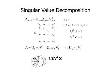
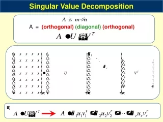
Singular Value Decomposition • If A is a rectangular m £ k matrix of real numbers, then there exists an m £ m orthogonal matrix U and a k £ k orthogonal matrix V such that • is an m £ k matrix where the (i, j)th entry i¸ 0, i = 1 min(m, k) and the other entries are zero • The positive constants i are the singular values of A • If A has rank r, then there exists r positive constants 1, 2,r, r orthogonal m £ 1 unit vectors u1,u2,,ur and r orthogonal k £ 1 unit vectors v1,v2,,vr such that • Similar to the spectral decomposition theorem
Singular Value Decomposition (contd.) • If A is a symmetric and positive definite then • SVD = Eigen decomposition • EIG(i) = SVD(i2) • Here AAT has an eigenvalue-eigenvector pair (i2,ui) • Alternatively, the vi are the eigenvectors of ATA with the same non zero eigenvalue i2
Example for SVD • Let A be a symmetric, positive definite matrix • U can be computed as • V can be computed as
Example for SVD • Taking 21=12 and 22=10, the singular value decomposition of A is • Thus the U, V and are computed by performing eigen decomposition of AAT and ATA • Any matrix has a singular value decomposition but only symmetric, positive definite matrices have an eigen decomposition
Applications of SVD in Linear Algebra • Inverse of a n £ n square matrix, A • If A is non-singular, then A-1 = (UVT)-1= V-1UT where -1=diag(1/1, 1/1,, 1/n) • If A is singular, then A-1 = (UVT)-1¼V0-1UT where 0-1=diag(1/1, 1/2,, 1/i,0,0,,0) • Least squares solutions of a m£n system • Ax=b (A is m£n, m¸n) =(ATA)x=ATb )x=(ATA)-1ATb=A+b • If ATA is singular, x=A+b¼ (V0-1UT)b where 0-1 = diag(1/1, 1/2,, 1/i,0,0,,0) • Condition of a matrix • Condition number measures the degree of singularity of A • Larger the value of 1/n, closer A is to being singular http://www.cse.unr.edu/~bebis/MathMethods/SVD/lecture.pdf
Applications of SVD in Linear Algebra • Homogeneous equations, Ax = 0 • Minimum-norm solution is x=0 (trivial solution) • Impose a constraint, • “Constrained” optimization problem • Special Case • If rank(A)=n-1 (m ¸ n-1, n=0) then x=vn ( is a constant) • Genera Case • If rank(A)=n-k (m ¸ n-k, n-k+1== n=0) then x=1vn-k+1++kvn with 21++2n=1 • Has appeared before • Homogeneous solution of a linear system of equations • Computation of Homogrpahy using DLT • Estimation of Fundamental matrix For proof: Johnson and Wichern, “Applied Multivariate Statistical Analysis”, pg 79
What is the use of SVD? • SVD can be used to compute optimal low-rank approximations of arbitrary matrices. • Face recognition • Represent the face images as eigenfaces and compute distance between the query face image in the principal component space • Data mining • Latent Semantic Indexing for document extraction • Image compression • Karhunen Loeve (KL) transform performs the best image compression • In MPEG, Discrete Cosine Transform (DCT) has the closest approximation to the KL transform in PSNR
Image Compression using SVD • The image is stored as a 256£264 matrix M with entries between 0 and 1 • The matrix M has rank 256 • Select r ¿ 256 as an approximation to the original M • As r in increased from 1 all the way to 256 the reconstruction of M would improve i.e. approximation error would reduce • Advantage • To send the matrix M, need to send 256£264 = 67584 numbers • To send an r = 36 approximation of M, need to send 36 + 36*256 + 36*264 = 18756 numbers • 36 singular values • 36 left vectors, each having 256 entries • 36 right vectors, each having 264 entries Courtesy: http://www.uwlax.edu/faculty/will/svd/compression/index.html