Download
1 / 27
270 likes | 544 Views
A PSE for Automatic Matlab 3D Finite Element Code Generation and Simplified Grid Computing. Zhou Jun, and Yukio Umetani Shizuoka University of Japan. Outline. Motivation Previous work Automatic Matlab 3D FEM code generation Execution of Matlab script via UNICORE

E N D
A PSE for Automatic Matlab 3DFinite Element Code Generation and Simplified Grid Computing Zhou Jun, and Yukio Umetani Shizuoka University of Japan
Outline • Motivation • Previous work • Automatic Matlab 3D FEM code generation • Execution of Matlab script via UNICORE • Conclusions and future work
Motivation • Interface to Matlab • popular for matrix computation • visualization facility • verifying simulation results of PSILAB • Reduce Matlab FEM programming effort • coding time • learning time • programming errors • Run Matlab script on the Grid via UNICORE
Internet GridPSi overview PSILAB PSILAB MATLAB Local Machine Internet Unicore Client GridPSi Client GridPSi Server Unicore Gateway Remote Server Usite NJS GridPSi Server TSI GridPSi Server GridPSi client connects GridPSi server in three ways.
GridPSi client arcitecture MATLAB Script Generator & Self-designed Matlab Functions PSILAB Script Generator
Automatic generation of Matlab 3D FEM code • MATLAB Script Generator • Self-coded Matlab functions PSILAB Script Generator Matlab Script Generator Generic Data structures Self-coded Matlab functions
Example problem To investigate the vertical movements at the bridge area of a 3D piano soundboard of simplified shape that is subjected to vertical pressures caused by the vibrations of the strings. (The soundboard is in anisotropic material)
Mathematical model • Governing equations: MÜ + CÙ + KU = R (1) • External forces: (2) • Boundary conditions: • Fixed Dirichlet conditions on the four sides • Generalized Neumann conditions on the top and bottom • Initial conditions: No displacements at the initial state
Finite element solution • Solid linear tetrahedron elements • Central difference method
Matlab FEM data structures Nodal coordinate matrix Element connectivity matrices • Problem domain • Boundary regions stiffness, mass, and damping matrices Nodal force vector Surface tractions (Neumann boundary condition) Unknown field on boundaries (Dirichlet condition)
Build nodal coordinate and element connectivity matrices function [node, setS, setV] = gmsh2matlab(‘meshFile’) • node: a matrix of nodal coordinates (n-by-3) • setS: a set of element connectivity matrices of boundary surfaces • setV: a set of element connectivity matrices of the volume(s) • meshFile: The input mesh file
Build stiffness matrix function[K] = buildStiffnessMatrix3D(node, elemV, E) (3) E: the consistent stress-strain compliance matrix function [E] = buildComplianceMatriceElastic3D(material properties) nG, Wk: integration point and weight function[W,Q] = quadrature(order,type,dimension) Jk: the determinant of the Jacobian matrix Bk: the bar matrix of the element function [N,dNdxi]=lagrange_basis('H4',pt)%return the Lagrange interpolant basis %and its gradients
function [K] = buildStiffnessMatrix3D(node, elemV, E) n = size(node,1);% get the total node number ‘n’. m = size (ElemV,1);% get the total element number ‘m’. K =sparse (3*n,3*n);% create the sparse global stiffness matrix ‘K’. for e = (1:m) % loops over the elements. str = ElemV(e,:); % get the four nodes comprising the current element. % the following is to build the Bar array ‘strBK’, which is used to locate the positions % of the four nodes in theglobal stiffness matrix. strBk = [str(1) str(1)+n str(1)+2*n str(2) str(2)+n str(2)+2*n ... str(3) str(3)+n str(3)+2*n str(4) str(4)+n str(4)+2*n]; [W,Q] = quadrature(1,'TRIANGULAR',3); % A function call returns the quadratrue weight W and Q for q = 1:size(W,1) pt = Q(q,:); wk = W(q); [N,dNdxi]=lagrange_basis('H4',pt);% A function call returns the lagrange interpolant basis. Jacobian = node(str,:)'*dNdxi;% get the Jacobian matrix. dNdX = dNdxi * inv(Jacobian); % a 4-by-3 matrix of the shape functions. %% construct the stress-displacement matrix BK (a 6-by-12 matrix) %% Bk = [dNdX(1,1) 0 0 dNdX(2,1) 0 0 dNdX(3,1) 0 0 dNdX(4,1) 0 0; 0 dNdX(1,2) 0 0 dNdX(2,2) 0 0 dNdX(3,2) 0 0 dNdX(4,2) 0; 0 0 dNdX(1,3) 0 0 dNdX(2,3) 0 0 dNdX(3,3) 0 0 dNdX(4,3); dNdX(1,2) dNdX(1,1) 0 dNdX(2,2) dNdX(2,1) 0 dNdX(3,2) dNdX(3,1) 0 dNdX(4,2) dNdX(4,1) 0; 0 dNdX(1,3) dNdX(1,2) 0 dNdX(2,3) dNdX(2,2) 0 dNdX(3,3) dNdX(3,2) 0 dNdX(4,3) dNdX(4,2); dNdX(1,3) 0 dNdX(1,1) dNdX(2,3) 0 dNdX(2,1) dNdX(3,3) 0 dNdX(3,1) dNdX(4,3) 0 dNdX(4,1)]; K(strBk,strBk) = K(strBk,strBk) + Bk’ *E * Bk * wk * det(Jacobian); % assemble the global matrix. end end
Build mass and damping matrices function [M] = buildMassMatrix3D(node, elemV ,rho) (4) (the integral over the element)
Enforce boundary conditions • Dirichlet boundary conditions: function [v] = applyEssentialBCs(v,node,elemS,id,dx,dy,dz) u t+1 = u t + 2Δt*v; % update displacement vector (5) • Neumann boundary conditions: function [f]=calculateSurfaceTraction(node,elemS,id,px,py,pz) R = f body + f surface traction1 + f surface traction2 + …
Initial Conditions function [Uold,Unow]= initalizeDisVectors(Uold,Unow,initU,initV) • Uold : the displacement vector at time t-1 • Unow : the displacement vector at time t • initU : the initial value at time -1 • initV : the initial value at time 0
Solution Scheme while (CT <500) t = t+delt; CT = CT+1; % Apply the Neumann conditions on given surfaces. [f1] = caculateSurfaceTraction2(node,elemS30,'30',0,0,-sz); [f2] = caculateSurfaceTraction2(node,elemS8,'8',0,0,0); R = f + f1 + f2; Unew = (a0*M+a1*C)\(Feffective - (K-a2*M)*Unow - (a0*M-a1*C)*Uold); Vnow = a1 * (Unew - Uold); % Apply the Dirichlet conditions on given surfaces. [Vnow] = applyEssentialBCs(Vnow,node,elemS17,'17',0,0,0); [Vnow] = applyEssentialBCs(Vnow,node,elemS21,'21',0,0,0); [Vnow] = applyEssentialBCs(Vnow,node,elemS25,'25',0,0,0); [Vnow] = applyEssentialBCs(Vnow,node,elemS29,'29',0,0,0); Unew = a3 * Vnow +Uold; Uold = Unow; Unow = Unew; Uzz = Unew([2*n+1:3*n],1);% get the displacements in Z direction. end % fid =fopen('matlabResults.txt','w'); fwrite(fid,Uzz); fclose(fid);
Executing Matlab script via UNICORE • Use of Script Task plug-in interface of UNIOCRE client • Preparation of a Job containing two tasks with dependency 1. script task: • command:matlab -nosplash -nodesktop -nodisplay -r soundboard • import files:the generated script, predefined Matlab functions, the mesh file 2. Export task: retrieve the simulation results back
Visual Effects of the Results Results solved by MATLAB Results solved by PSILAB
Correctness In the same iteration step, at the same integration point, the values of the small displacements on the top of the soundboard solved by Matlab and PSILAB are: • in the same order (10-10); • the first three digitals of the values are almost the same
Related Works PDE Toolbox (MathWorks) • Only supports 1D and 2D PDE-based problems; Geodise (University of Southampton) • Uses MATLAB as a scripting language engine; • Users need to program MATLAB. FEMLAB (COMSOL Inc.) •Does not support Grid access GridPSi •Supports real-world 2D and 3D PDE-based problems; • Automatic generation MATLAB script without programming; • Grid accessible.
Conclusions • Layered architecture and component-based design makes our system easily interface to Matlab. • Automatic Matlab FEM code generation greatly reduces users’ work and programming errors. • Simple Grid access pattern lowers barriers to enter for users who wish to run their physical simulations on the Grid.
Future Work • The real-time visualization through Unicore/VISIT and AVS/Express • The design of nonlinear PDE Wizards