Download
1 / 12
130 likes | 229 Views
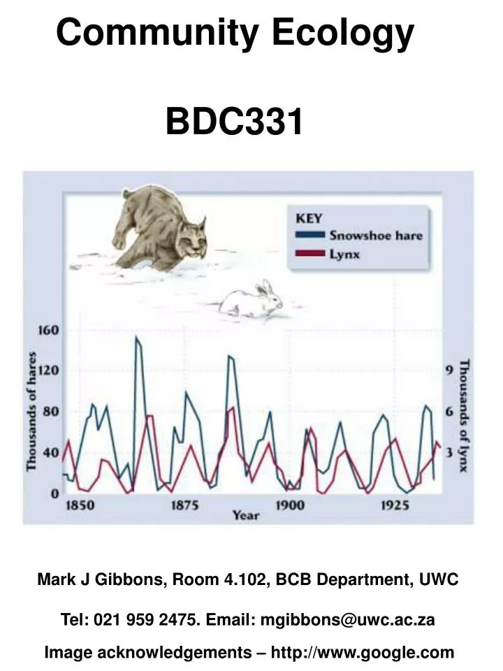
Community Ecology BDC331. Mark J Gibbons, Room 4.102, BCB Department, UWC Tel: 021 959 2475. Email: mgibbons@uwc.ac.za. Image acknowledgements – http://www.google.com. Southern (1970) J Zoology 162: 197-285. Not always an obvious relationship between predator and prey.

E N D
Community Ecology BDC331 Mark J Gibbons, Room 4.102, BCB Department, UWC Tel: 021 959 2475. Email: mgibbons@uwc.ac.za Image acknowledgements – http://www.google.com
Southern (1970) J Zoology 162: 197-285 Not always an obvious relationship between predator and prey Dempster & Lakhani (1979) J Animal ecology 48: 143-164 Sometimes…..
Nt+1 = Nt + r.Nt – a.Pt.Nt d N d N Nt+1 - Nt d t d t Intrinsic rate of natural increase t1 – t0 = 1 = r.N – a.P.N Modeling Predator Prey Dynamics Lotka-Volterra For populations displaying continuous breeding = r.N Exponential Growth N = number of prey Prey individuals are removed at a rate that depends on the frequency that predators encounter prey. Encounters increase with predator (P) and prey (N) numbers. The exact numbers encountered and actually consumed will depend on the searching and attack efficiency of the predator (a) – aPN
* Nt+1 = Nt + r.Nt – a.Pt.Nt = – q.P * Pt+1 = Pt + f.a.Pt.Nt– q.Pt = f.a.P.N– q.P d P d P d N d t d t d t Lotka-Volterra equations COPY THESE EQUATIONS = r.N – a.P.N In the absence of prey, predator numbers will decline exponentially through starvation Where q = predator mortality rate Counteracted by predator birth – assumed to depend only on the rate at which food is consumed (a.P.N) and the efficiency (f) at which a predator converts this to offspring
dN = Nt+1 - Nt dN dN dN = r.Nt – a.Pt.Nt IF = 0 = 0 dt dt dt 0 = r.Nt – a.Pt.Nt Then r.Nt = a.Pt.Nt Dividing by Nt r = a.Pt Dividing by a r/a = Pt Nt+1 = Nt + r.Nt – a.Pt.Nt Equilibrium Solutions What is the population size of the predators that induces no change in the prey population size NOTE –This is a constant. Prey population size at EQUILIBRIUM not determined by this solution – population size can be stable at any size as long as predator population at specified size
dP = Pt+1 - Pt dP dP dP = -q.Pt + a.f.Pt.Nt IF = 0 = 0 dt dt dt 0 = -q.Pt + a.f.Pt.Nt Then q.Pt = a.f.Pt.Nt Dividing by Pt q = a.f.Nt Dividing by a.f q/a.f = Nt Pt+1 = Pt - q.Pt + a.f.Pt.Nt Equilibrium Solutions What is the population size of the prey that induces no change in the predator population size NOTE – This is a constant. Predator population size at EQUILIBRIUM not determined by this solution – population size can be stable at any size as long as prey population at specified size
dN = 0 dt When r/a = Pt r/a Predator Population Prey Population Prey populations will increase in size at predator densities less than r/a, but will decrease in size at predator densities greater than r/a
dP = 0 dt When q/a.f = Nt Predator Population q/a.f Prey Population Predator populations will increase in size at prey densities greater than q/a.f, but will decrease in size at prey densities less than q/a.f
r/a Predator Population q/a.f Prey Population r/a Predator Population q/a.f Prey Population Combining the two equilibria
Open a spreadsheet in MSExcel Nt+1 = Nt + r.Nt – a.Pt.Nt Pt+1 = Pt + f.a.Pt.Nt– q.Pt BUT……….. MUST constrain BOTH populations so that if numbers drop to zero, they remain at zero. Use an IF argument =IF(G2+(B$4*G2)-(D$4*H2*G2)>0, (G2+(B$4*G2)-(D$4*H2*G2),0) How do different values of r, a, q,N0, P0, and f influence the outcomes of species interactions? Next – Project a prey and a predator population into the future for 100 time units – using these two equations
Plot predator and prey numbers on an X-Y graph It should look something like this: Coupled Oscillations Plot the two populations on a line graph It should look something like this: Coupled Oscillations
THE END Image acknowledgements – http://www.google.com