Download
1 / 58
630 likes | 890 Views
THE WATERSHED SEGMENTATION. NADINE GARAISY. GENERAL DEFINITION.

E N D
THEWATERSHED SEGMENTATION NADINE GARAISY
GENERAL DEFINITION A drainage basin or watershed is an extent or an area of land where surface water from rain melting snow or ice converges to a single point at a lower elevation, usually the exit of the basin, where the waters join another waterbody, such as a river, lake, wetland, sea, or ocean
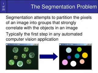
INTRODUCTION • The Watershed transformation is a powerful tool for image segmentation, it uses the region-based approach and searches for pixel and region similarities. • The watershed concept was first applied by Beucher and Lantuejoul at 1979, they used it to segment images of bubbles and SEM metallographic pictures
IMAGE REPRESENTATION • We will represent a gray-tone image by a function: is the gray value of the image at point • A section of at level is a set defined as: And in the same way we define as: =
REMINDER-IMAGE GRADIENT An image gradient is a directional change in the intensity or color in an image. Image gradients may be used to extract information from images.
IMAGE GRADIENT a gradient image in the x direction measuring horizontal change in intensity a gradient image in the y direction measuring vertical change in intensity an intensity image
IMAGE GRADIENT • The morphological gradient of a picture is defined as Where is the dilation of and is its erosion. But because is continuously differentiable, is nothing more than the modulus of the gradient of
GEODESIC DISTANCE • For two points when we define the geodesic distance as the length of the shortest path (if any) included in and linking and • Let be any set included in , then: • is the set of all points of that are at a finite geodesic distance from
GEODESIC ZONE OF INFLUENCE • The geodesic zone of influence of (when is composed of connected components ) is the set of points inwhose finite distance is closest to (among all components)
GEODESIC SKELETON BY ZONES OF INFLUENCE • The boundaries between the various zones of influence give the geodesic skeleton by Zones of influence of in
MINIMA AND MAXIMA • The set of points in the function can be seen as topographic surface , The lighter the gray value of the function at the point the higher the altitude of the corresponding point on the surface
MINIMA AND MAXIMA • An ascending path is a sequence On the surface such that: • A point belongs to a minimum if there is a no ascending path starting from . It can be considered as a sink of the topographic surface (see next slide). The set of all the minima of is made of various connected components
THE WATERSHED TRANSFORMATION If we look at the image as a topographic surface, imagine that we pierce each of the topographic surface and then we plunge this surface into a lake, the water entering through the holes floods the surface and if two or more floods coming from different minima attempt to merge, we avoid this event by building a dam on the points of the surface where the floods would merge. At the end of the process only these dams will emerge and this is what define the watershed of the function
THE WATERSHED TRANSFORMATION • http://cmm.ensmp.fr/~beucher/lpe1.gif
BUILDING THE WATERSHED • Suppose the flood of the surface has reached the section , when it continue and reach the flooding is performed in the zones of influence . • The components of which are not reached by the flood are the minima at this level and must be added to the flooded area
BUILDING THE WATERSHED • If we define as the catchment basins of at level and as the minima of at height then: • The initiation of this iterative algorithm is • In the end the watershed line is when • Visual illustration
OVER-SEGMENTATION PROBLEM Unfortunately, most times the real watershed transform of the gradient present many catchment basins, Each one corresponds to a minimum of the gradient that is produced by small variations, mainly due to noise.
OVER-SEGMENTATION: SOLUTION The over-segmentation could be reduced by appropriate filtering, but the best results is obtained by marking the patterns to be segmented before preforming the watershed transformation of the gradient.
OVER-SEGMENTATION: SOLUTION FIRST: we mark each blob of protein of the original image (by extracting the minima of the image function)
OVER-SEGMENTATION: SOLUTION • SECOND: by applying the watershed on the initial image we can mark the background with connected marker surrounding the blobs • We define these two steps as marker set
HOMOTOPY MODIFICATION The first two steps of this algorithm can be done by modifying the gradient function to a new wery similar function , the difference between the two is that in the initial minima are replaced by the set this modification is called homotopy modification
OVER-SEGMENTATION: SOLUTION Now we look at the final result of the marking as a topographic surface, but in the flooding process instead of piercing the minima, we only make holes through the components of the marker set that we produced The initial image marked with the set
OVER-SEGMENTATION: SOLUTION This way the flooding will produce as many catchment basins as there are markers in this way the watershed lines of the contours of the objects will be on the crest lines of this topographic surface
OVER-SEGMENTATION: SOLUTION • The algorithm for this solution is as follows: – section at level of the new catchment basins of Then: Initialization:
OVERLAPING GRAINS • In some cases we have an image with overlapping figures, that we need to segment, in order to do that we need to point out the overlapping regions. • For example the figure here is a TEM (transmission electron microscopy) image of grains of silver nitrate scattered on a photographic plate.
OVERLAPING GRAINS To point out the overlapping regions we first threshold the initial image to a binary image with only two gray values
REMINDER: DISTANCE FUNCTION • the distance function of an image assigns for each pixel a number that is the Euclidean distance between that pixel and the nearest nonzero pixel. • For example: suppose we have this image matrix- • Then the distance matrix will be-
OVERLAPING GRAINS By calculation the maxima of the distance function of the binary image we can provide the markers of the grains
OVERLAPING GRAINS The markers of the overlapping regions are obtained by executing the watershed transformation of the inverted distance function it will produce divide lines which will cut the overlapping grains, that way we can mark them.
OVERLAPING GRAINS Finally after marking the background and calculation the gradient function we run the homotopy modification and the watershed construction are preformed
THE SEGMENTATION PARADIGM The segmentation process is divided into two steps: Finding the markers and the segmentation. Performing a marker-controlled watershed with these two elements
WATERSHED TRANSFOTMATION PROCESS Step 1: Use the Gradient Magnitude as the Segmentation Function - The gradient is high at the borders of the objects and low (mostly) inside the objects. Source: A gray scale image Step 2: Mark the foreground objects from - www.mathworks.com
WATERSHED TRANSFOTMATION PROCESS Step 5: Calculate the regional maxima to obtain good foreground markers. Step 3: computing the opening-by-reconstruction of the image Step 4: Following the opening with a closing can remove the dark spots and stem marks. from - www.mathworks.com
WATERSHED TRANSFOTMATION PROCESS Step 6: Superimpose the foreground marker image on the original image, Notice that the foreground markers in some objects go right up to the objects' edge Step 8: Compute Background Markers, Starting with thresholding operation Step 7: cleaning the edges of the marker blobs and then shrinking them a bit from - www.mathworks.com
WATERSHED TRANSFOTMATION PROCESS Step 9: Compute Background Markers, using the watershed transform of the distance transform and then looking for the watershed ridge lines of the result Step 10: Visualize the Result, one of the techniques is to superimpose the foreground markers, background markers, and segmented object boundaries. from - www.mathworks.com
WATERSHED TRANSFOTMATION PROCESS – ADVANCE OPTIONS We can use transparency to superimpose this pseudo-color label matrix on top of the original intensity image. *Another useful visualization technique is to display the label matrix as a color image from - www.mathworks.com
ROAD SEGMENTATION • In this study they use the watershed algorithm among others to extract vehicle position on the road and possible obstacles ahead. • The algorithms have been tested on a small database representing different driving situations.
ROAD SEGMENTATION The original road image The morphological gradient image
ROAD SEGMENTATION Due to noise and inhomogeneities in the gradient image, the watershed will produce a lot of minima which leads to over-segmentation of the image
ROAD SEGMENTATION We can enhance the watershed on the gradient image by modifying the gradient function by defining new markers which will be imposed as the new minima.
ROAD SEGMENTATION The difference between watershed on simple gradient and watershed on the gradient after modifying using the regularized gradient
ROAD SEGMENTATION Then by selecting the catchment basin located at the front of the vehicle we can extract a coarse marker of the road. After smoothing this marker we define it as
ROAD SEGMENTATION Then we build an outer marker to mark the region of the image which do not belong to the road This marker is defined by
ROAD SEGMENTATION Using and we modify the gradient which now contain only two minima and the divide lines are the contours of the road
ROAD SEGMENTATION • To obtain the road markers we do a simplification on the image using its gradient, the result is an image made of catchment basins tiles of constant gray values- this image is called the mosaic-image. • The gradient of this image will be null everywhere except on the divide lines where it will be equal to the absolute difference of the gray-tone values of the to catchment basins.
ROAD SEGMENTATION Watershed of the mosaic-image points out only the regions surrounded by higher contrast edges, and we can still extract a marker for the road