Download
1 / 84
840 likes | 883 Views
Learn about the zeros and poles of transfer functions in control systems and their significance. Understand the time response of first and second-order systems. MATLAB simulations included.

E N D
Time Response*, ME451 Instructor: Jongeun Choi * This presentation is created by Jongeun Choi and Gabrial Gomes
Zeros and poles of a transfer function • Let G(s)=N(s)/D(s), then • Zeros of G(s) are the roots of N(s)=0 • Poles of G(s) are the roots of D(s)=0 Im(s) Re(s)
Theorems • Initial Value Theorem • Final Value Theorem • If all poles of sX(s) are in the left half plane (LHP), then
DC gain or static gain of a stable system 1.4 1.2 1 0.8 0.6 0.4 0.2 0 0 0.5 1 1.5 2 2.5 3
DC Gain of a stable transfer function • DC gain (static gain) : the ratio of the steady state output of a system to its constant input, i.e., steady state of the unit step response • Use final value theorem to compute the steady state of the unit step response
Pure integrator • ODE : • Impulse response : • Step response : • If the initial condition is not zero, then : Physical meaning of the impulse response
First order system • ODE : • Impulse response : • Step response : • DC gain: (Use the final value theorem)
First order system • If the initial condition was not zero, then Physical meaning of the impulse response
Matlab Simulation • G=tf([0 5],[1 2]); • impulse(G) • step(G) • Time constant
First order system response System transfer function :
First order system response System transfer function : Impulse response :
First order system response System transfer function : Impulse response :
First order system response System transfer function : Impulse response : Step response :
First order system response Im(s) Re(s)
First order system response Im(s) Unstable Re(s)
First order system response Im(s) Unstable Re(s) -1
First order system response Im(s) Unstable Re(s) -2
First order system response Im(s) Unstable faster response slower response Re(s) constant
Time to go from to First order system – Time specifications. Time specs: Steady state value : Time constant : Rise time : Settling time :
First order system – Simple behavior. No overshoot No oscillations
Second order system (mass-spring-damper system) • ODE : • Transfer function :
Polar vs. Cartesian representations. Cartesian representation : … Imaginary part (frequency) … Real part (rate of decay)
Polar vs. Cartesian representations. Cartesian representation : … Imaginary part (frequency) … Real part (rate of decay) Polar representation : … natural frequency … damping ratio
Polar vs. Cartesian representations. Cartesian representation : … Imaginary part (frequency) … Real part (rate of decay) Polar representation : … natural frequency … damping ratio
Polar vs. Cartesian representations. Cartesian representation : … Imaginary part (frequency) … Real part (rate of decay) Polar representation : … natural frequency … damping ratio Unless overdamped
Polar vs. Cartesian representations. System transfer function : Significance of the damping ratio : … Overdamped … Critically damped … Underdamped … Undamped
Polar vs. Cartesian representations. System transfer function : Significance of the damping ratio : … Overdamped … Critically damped … Underdamped … Undamped
Polar vs. Cartesian representations. System transfer function : Significance of the damping ratio : … Overdamped … Critically damped … Underdamped … Undamped
Polar vs. Cartesian representations. System transfer function : All 4 cases Unless overdamped Significance of the damping ratio : … Overdamped … Critically damped … Underdamped … Undamped
Underdamped second order system • Underdamped • Two complex poles:
Matlab Simulation • zeta = 0.3; wn=1; • G=tf([wn],[1 2*zeta*wn wn^2]); • impulse(G)
Unit step response of undamped systems • Unit step response : • DC gain :
Matlab Simulation • zeta = 0.3; wn=1; G=tf([wn],[1 2*zeta*wn wn^2]); • step(G)
Second order system response. Stable 2nd order system: 2 distinct real poles A pair of repeated real poles A pair of complex poles Im(s) Unstable Re(s)
Second order system response. Stable 2nd order system: 2 distinct real poles A pair of repeated real poles A pair of complex poles Im(s) Unstable Re(s)
Second order system response. Stable 2nd order system: 2 distinct real poles A pair of repeated real poles A pair of complex poles Im(s) Unstable Re(s)
Second order system response. Stable 2nd order system: 2 distinct real poles A pair of repeated real poles negative real part A pair of complex poles zero real part Im(s) Unstable Re(s)
Second order system response. Stable 2nd order system: 2 distinct real poles A pair of repeated real poles negative real part A pair of complex poles zero real part Im(s) Unstable Re(s)
Second order system response. Stable 2nd order system: 2 distinct real poles A pair of repeated real poles negative real part A pair of complex poles zero real part Im(s) Unstable Re(s)
Second order system response. Im(s) 2 distinct real poles = Overdamped Unstable Re(s)
Second order system response. Im(s) Repeated real poles = Critically damped Unstable Re(s)
Second order system response. Im(s) Complex poles negative real part = Underdamped Unstable Re(s)
Second order system response. Im(s) Complex poles zero real part = Undamped Unstable Re(s)
Second order system response. Im(s) Underdamped Unstable Undamped Overdamped or Critically damped Re(s) Underdamped
Overdamped system response System transfer function : Impulse response : Step response :