Download

1 / 34
350 likes | 457 Views
RHIC Luminosity Increase with Bunched Beam Stochastic Cooling. M. Blaskiewicz , J.M. Brennan, K. Mernick C-AD BNL Michaela Schaumann CERN Acknowledgements Dave McGinnis (ESS), Ralph Pasquinelli (FNAL)

E N D
RHIC Luminosity Increase with Bunched Beam Stochastic Cooling M. Blaskiewicz, J.M. Brennan, K. Mernick C-AD BNL Michaela Schaumann CERN Acknowledgements Dave McGinnis (ESS), Ralph Pasquinelli (FNAL) Fritz Caspers, Flemming Pedersen, John Jowett (CERN) Wolfram Fischer, Vladimir Litvinenko, Derek Lowenstein, Thomas Roser (BNL) Jie Wei (FRIB) Instrumentation, Controls and RF groups at BNL • History • The RHIC System • Results and Comparison with Simulations
History Herr and Mohl reported cooling bunched beams in ICE (1978) Chattopadhyay develops bunched beam cooling theory (1983) Stochastic cooling considered for SPS, RHIC and Tevatron (80s). Unexpected RF activity swamps the Schottky signal (85s). Boussard et.al. use channels for data transmission. Signal Suppression in the Tevatron (95). Cooling of long bunches in FNAL recycler, mixing via IBS. Proton cooling experiment in RHIC (2006). Operational longitudinal cooling of gold in RHIC (2007). Transverse cooling in RHIC (2010). Solution of cross talk problem by cavity frequency offset (2011). Full 3-D cooling in RHIC (2012).
Voltage considerations For 6-9 GHz longitudinal system we need 3 kV rms. Bandwidth-Voltage product sets the cost scale. Bunches are 5 ns long spaced by 100 ns. The value of the kicker voltage matters only when the bunch is present.
Error Limit Simulations Took conservative errors. • 2 ps timing error • 20% amplitude errors • 2 MHz cavity frequency errors Desired cooling voltage is modeled as band limited noise. System is well behaved with these errors.
Voltage and Power continued Take 16 cavities, 6-9 GHz bandwidth 40 Watts/cavity R/Q=100, 10 MHz FWHP bandwidth, R 50 kilo-Ohm gives 1 to 1.4 kV rms per cavity, or 5.6 kV total Cavity drive signal needs to be roughly sinusoidal for R (not R/Q) to matter Suppose is the drive signal for a broad band kicker (like a resistor). Periodically extend This creates a signal spectrum with peaks spaced by with width Split and pass through 100 MHz filters, centered on cavity resonance, before power amps. In this way each amplifier sees a piecewise sinusoidal input. Combination of transmission lines and fiber optic technology for the delay line (traversal) filter.
Transverse Cooling system Panofsky-Wenzel theorem relates transverse kick to standard voltage Similar cavities. 40 Watt amplifiers are sufficient. 4.8-7.8 GHz keeps aperture reasonable. 2b
The RHIC system layout Longitudinal cooling uses 70 GHz microwave links. Transverse cooling uses fiber optics. Yellow transverse 4.8,5.0,..7.8 Blue transverse 4.7,4.9,..7.7 to avoid cross-talk through IRs
Integrated uranium luminosity improved 5 fold with cooling. Is it what we deserve?
Quick reminder of how stochastic cooling works perfect mixing • So, reducing N increases cooling rate. • A simulation with M<N macro-particles reaches the same macroscopic parameters in M/N the updates. M < 10-3 N
Bunched Beam Simulations Time domain model of filter cooling. Very similar to coherent stability problem. Need to have pickups and kickers in different locations to correctly account for phase slip and betatron phase advance. Signal to noise addressed by adding noise in the pickup. 200 MHz cavity spacing addressed by folding all data into 5 ns interval before FFT and convolution. Need to add IBS, which is done as random kicks modulated by line density.
Transverse Cooling Simulations Check of scaling, single harmonic rf, no IBS or longitudinal cooling
Intra-beam scattering helps transverse cooling IBS causes diffusion in longitudinal action. Physically important for FNAL Recycler, it’s a major source of mixing. For RHIC, longitudinal cooling keeps the distribution in the bucket, but a given particle will wander in synchrotron amplitude. The net effect is that all particles have good transverse cooling. This gives a new simulation time scale to worry about. One must make sure that the fast mixing from IBS is small compared to the fast mixing from synchrotron motion.
Inclusion of burn-off (luminosity losses) Spatial density for gaussian beam traveling to left Particle traveling to right Probability particle interacts Average over betatron phase
Uranium beam size reduced 2.2x10⁸ U ions ɛn=0.23 µm
Longitudinal evolution for uranium • Dual harmonic RF Profiles each hour
Luminosity evolution with constant gain • Integrals agree within 1%
Full cooling more than doubles integrated luminosity for typical gold intensities.
Updating longitudinal kickers to scissor design. 2x3 Cell longitudinal kickers increase voltage. Waveguide coupler eliminates coaxial cables. Prototyping in progress.
Considerations for LHC Took 2/3 turn delay and single one turn delay filter.
Voltage and power Considerations, 1GHz cavity spacing Results from simulations give near optimal luminosity For 2kV rms, which was adopted. With 1 GHz spacing the voltage per cavity does not depend on band width at 12 GHz
Voltage and power 2 Our cavities typically have R/Q = 100 Ohm (circuit def.) At 12 GHz Q = 600 for 20 MHz band width, R=60kOhm Power = (Vrms)2/R=66 Watts, rms. Probably want 200 or more watts. Saturation can be simulated (but not yet). Limiters that saturate without introducing a phase shift would be very useful. Transverse voltage of 200 V rms per cavity. Need to follow up on power requirements.
Conclusions • First implementation of 3D cooling in a collider worked as predicted. • Integrated luminosity in U-U improved 5 fold. • Cooling led to first increase of instantaneous luminosity and smallest emittance ever in a hadron collider. • Simulations have adequate predictive power to design with confidence. • For 1.3E9/bunch, cooling will improve integrated luminosity by a factor of 2 or more, system allows operation up to 2.E9/bunch • 56 MHz yields an additional 30 to 50% luminosity depending on vertex cut. • Preliminary results for LHC are promising.
Au luminosity versus acceptance 2x10⁹ 1x10⁹