Chap 5: Classical Magnetic dipole moment 

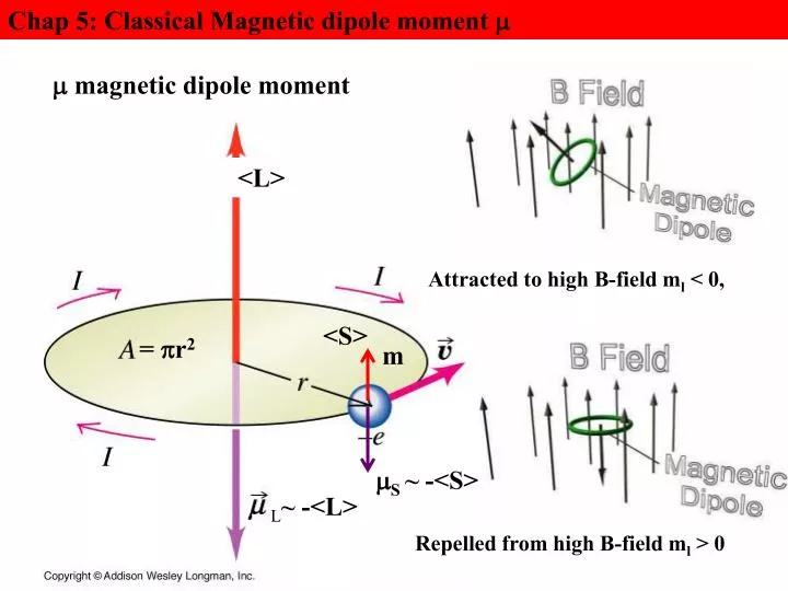
Chap 5: Classical Magnetic dipole moment   magnetic dipole moment <L> Attracted to high B-field ml < 0, <S> = r2 m S ~ -<S> L~ -<L> Repelled from high B-field ml > 0

Chap. 5:H-atom and One electron Ions Eigen Functions and Values Ylm( Angular part of the eigen-functions for the Schrödinger Eq. are also the eigen functions for the Magnitude Squared of the total orbital angular momentum: L2 L2 Ylm(=l(l+1)h2Ylm( and the projection of the total orbital angular momentum vector along the z-axis: Lz Lz Ylm( = mhYlm(

Chap. 5:H-atom and One electron Ions Eigen Functions and Values Ylm( Angular part of the eigen-functions for the Schrödinger Eq. are also the eigen functions for the Magnitude Squared of the total orbital angular momentum: L2 L2 Ylm(=l(l+1)h2Ylm( and the projection of the total orbital angular momentum vector along the z-axis: Lz Lz Ylm( = mhYlm( B=Baz Magnetic Field B

Chap. 5:H-atom and One electron Ions Eigen Functions and Values Ylm( Angular part of the eigen-functions for the Schrödinger Eq. are also the eigen functions for the Magnitude Squared of the total orbital angular momentum: L2 L2 Ylm(=l(l+1)h2Ylm( and the projection of the total orbital angular momentum vector along the z-axis: Lz Ex: l = 2 Lz Ylm( = mhYlm( B=Baz m < 0 m < 0 Magnetic Field B

Chap. 5: Correspondence Principle and the Bohr Limit L=nh The Bohr limit only applies for l >>1 <|L|2>=L2 = l(l+1)h2  l2h2 for l >>1 the Bohr limit! Magnitude of L=√L2~ lh, l >>1 and the its z-axis projection <Lz>= Lz ~ lh (-h2/2m) ”nlm + V(r) nlm = Ennlm where nlm(r,,) = Rnl( r )Ylm( L2 Ylm(=l(l+1)h2Ylm( and Lz Ylm( = mhYlm( Therefore n, l, m and Encompletely characterizes a Quantum State along with Electron spin angular momentum!

Chap. 5: Correspondence Principle and the Bohr Limit L=nh Ex: Lz= -ih∂/∂ Lz operator Lz Ylm( = -ih∂(Ylm( /∂)= mhYlm( Therefore Ylm(~ exp(im) ∂(Ylm( /∂)= im Ylm( -ih∂(Ylm( /∂ = -ihim Ylm( Lz Ylm( = mhYlm( Eigen Value Eigen Function

Vector model of the Spin angular momentum s=1/2 s =1/2 is the spin angular momentum quantum number B||z repelled from stronger B-field ms=+1/2 <S>=Sz= msh S-spin angular momentum Vector x,y plane <|S|2>=S2 magnitude squared Of the Spin angular Momentum Vector S S2= s(s+1)h2 The magnitude √S2=√s(s+1)h2 ms=-1/2 attracted to stronger B-field

Chap 5: Classical Magnetic dipole moment   magnetic dipole moment <L> Attracted to high B-field ml < 0, <S> = r2 m S ~ -<S> L~ -<L> Repelled from high B-field ml > 0

Chap 5: Angular Momentum Eigen Values Vector model of t bare angular momentum L: only the Magnitude L and one component, Lx, Ly or Lzcan be measured! Magnitude Squared <|L|2>=L2=l(l+1)h2 z-axis projection Lz= mlh z Magnitude of L L= √l(l+1)h2 ml =+1 <L>=Lz= mlh L y ml =0 x L Ex. For: l= 1 2l + 1 ml –values 2(1)+1=3 ml =-1

Chap 5: Angular Momentum Eigen functions Ypz=Y10( z  x <Lz>=0 L Angular eigen function for the State l=1; m=0 Ypz=Y10(=√(3/4π) cos() Angular momentum Eigen Function + Phase L=√2 h + Notice that only Eigen Values are knowable, i.e., measurable: E, L2, Lz - - Phase Ypz=Y10(= √(3/4π) cos() |Y10(|2 =(3/4π) cos2()

Chap. Spherical Coordinate Sphere of Radius r

Chap 5: Angular Momentum Eigen functions Ypz= Ypz Ypy Ypz=Y10~cos() Linear Combinations of Eigen Functions Ypx=(1/√2){Y11 + Y1-1} ~ sin()cos() Ypy=(1/√2){Y11 - Y1-1} ~ sin()sin() Liner Superposition of states (l, m) in this Case of (l=1, m=+1) and (l=1, m=-1)

z y x |Y00|2 |Y1±1|2 |Y10|2

Chap. 5: 3-D Probability Density r|2dV =|R(r)Y()|2dV Probability per unit volume of finding the electron in the volume element: dV=dxdydz= {rd}{rsin(d}dr |R(r )|2 (r2dr) probability of finding the electron between a distance r and r+dr |R(r )|2 r2 Prob per unit length |Y()|2sin(dd= |Y()|2d probability of finding the electron in the solid angle d=sin(dd |Y()|2 Prob per unit solid angle Fig. 5-1, p. 171

Chap. Solid Angle for a Sphere of Radius r The solid angleddA/r2 = sin(dddV= dr dA(surface area of dV), dA = r2sin(dd A=4πr2(surface area of the sphere)r2 = 4π solid angle portended(projected) by a sphere dA Differentail Area

Chap 5: Angular Momentum Eigen functions Ypz= Ypz Ypy Ypz=Y10~cos() Linear Combinations of Eigen Functions Ypx=(1/√2){Y11 + Y1-1} ~ sin()cos() Ypy=(1/√2){Y11 - Y1-1} ~ sin()sin()

=Zr/a0 • Recall that the Bohr radii are rn= n2/Za0 Table 5-2, p. 175

Chap 5:1s ~R10( r ) Y00(, 2s~R20( r ) Y00(, 3s~R30( r ) Y00( Number of Nodes in Rnl (n-l-1): radial nodes l angular nodes a0 the Bohr is most probable radius Sphere Radius rs Prob < 0.05 of max prob for finding electron at r > rs

Chap 5:, 2pz~R20( r )Ypz(, 3pz R31( r )Ypz( Ypz ~ cos( |Ypz|2~ |cos( r  2pz~R20( r )Ypz( One electron orbital

Chap 5:, 2pz~R20( r )Ypz(, 3pz R31( r )Ypz( Ypz ~ cos( |Ypz|2~ |cos( r  L 2pz~R20( r )Ypz(

Chap 5:, 2pz~R20( r )Ypz(, 3pz R31( r )Ypz( 2pz~R20( r )Ypz( 2pz one electron orbital 2px~R21( r )Ypx( 2px one electron orbital 2py~R21( r )Ypy( 2py one electron orbital

Chap 5: Angular Momentum Eigen functions d-orbital L dzz ~ R32( r ) Y20( L r  r  L  dx2 -y2 ~ R32{Y22 +Y2-2}~cos(2) dxy ~ R32{Y22 - Y2-2}~ sin(2)

Chap 5: Aufbau Process; Atomic Ground State Electron Configuration P D P D P P P P P D

Chap 5: Periodic Table reflects the Electron Configuration; Atomic Properties Alkali Metals Rare Gases 2 8 Noble Metals Transition Metals 8 18 18 Halogens Alkaline earth Lanthanides Actinides

Chap 5: Periodic Table reflects the Electron Configuration: ionization Energies X X+ + e E=E(X+) - E(X)=IE1 and X+X2+ + e E=E(X2+) - E(X+)=IE2

Chap 5: Periodic Table reflects the Electron Configuration: ionization Energies

Chap 5: Periodic Table reflects the Electron Configuration: Electron Affinity X + e X-E = E(X-) - E(X)= - EA

Chap. 5:H-atom and One electron Ions Eigen Funct, and Values nlm(r,,) = Rnl( r )Ylm(: Eigen Function : Energy Eigen Values (same as Bohr) Principal quantum number Angular momentum quantum number Magnetic quantum number

Chap 5: Quantum Mechanical Energy levels The Energy Eigen Values are Independent of l and m! Therefore each n level has n, l levels (0,1, ..n-1), each with (2l+1) states and is therefore n2 degenerate. Consequently each (nl) level has (2l+1) m-states and is (2l+ 1) degenerate

Chap 5: Average QM distance of the electron from the Nucleus Chap 5: Average QM distance of the electron from the Nucleus The Average Quantum Mechanicaldistance between the Nucleus and the electron:<rnl> = (a0n2/Z){1+(1/2)[1- l(l+1)2/n2]}.For n>>1 and n~l reduces tothe Bohr Modelrn= (a0n2/Z) is also the most probable distance of the electron from the nucleusVisualizing atomic orbital probability density:http://www.phy.davidson.edu/stuhome/cabell_f/density.html The Average Quantum Mechanicaldistance between the Nucleus and the electron:<rnl> = (a0n2/Z){1+(1/2)[1- l(l+1)2/n2]}.For n>>1 and n~l reduces tothe Bohr Modelrn= (a0n2/Z) is also the most probable distance of the electron from the nucleusVisualizing atomic orbital probability density:http://www.phy.davidson.edu/stuhome/cabell_f/density.html

Vector model of the Spin angular momentum S=1/2 S =1/2 is the total spin quantum number B||z repelled from stronger B-field ms=+1/2 S-spin angular momentum <Sz>=Sz= msh x,y plane <|S|2>=S2= s(s+1)h2 z-axis projection <Sz>=Sz=msh ms=-1/2 attracted to stronger B-field

Chap 5: Classical Magnetic dipole moment 