Download
1 / 20
200 likes | 358 Views
Interarea Price Levels Bettina H. Aten Bureau of Economic Analysis. Outline . What are Interarea Levels? Why are they important? What difference would they make? How do you calculate them?. Interarea Price Levels. Measure price differences across space Reference place = 1.00

E N D
Interarea Price LevelsBettina H. AtenBureau of Economic Analysis
Outline What are Interarea Levels? Why are they important? What difference would they make? How do you calculate them?
Interarea Price Levels Measure price differences across space Reference place = 1.00 • Typically the National average • Each locality’s price level relative to the national
Area 1’s level = 1.10 → 10% more expensive • Area 2’s level = 0.95 → 5% less expensive • Area 1 is 15.8% more expensive than Area 2 (1.10 ÷ 0.95 = 1.158)
Unified Time and Place Index • National Index in base year = 100.0 • 2 – dimensional • Force consistency
U.S. = 1.00 New York = 1.27 Houston = 0.92 Boston = 1.15 Pittsburgh = 0.83 Chicago = 1.03 San Francisco = 1.35 Price Levels San Francisco’s price level is 62.5% > Pittsburgh’s = 16 or 17 years of inflation
Dramatic differences Personal Income per capita 2003 (Nominal Adjusted to Rank) Nominal US prices Mississippi (50) $23,448 $30,062 Hawaii (19) $30,913 $22,899 Miss. adjusted by the “C” South 0.78 Hawaii adjusted by Honolulu MSA 1.35
Prices ≈1 million price observations (Jan-Dec 2003) ≈ 230,000 annual average prices Unique by outlet, quote and version code geometric mean over months • Prices of consumers living in area • Not prices of the stores located in the areas
Weighted hedonic • Uses information from all areas • Weights the areas appropriately • Like a symmetric index formula Find price level relative for: each geographic area 38 areas and each item category 398 categories categories with prices 373 ≈ 15,000 price parities Aggregate using Country-Product-Dummy (CPD) method
Two Stages of Price Level Calculations • Price parities for each area and item category • Similar to elementary aggregates • One regression for each item category • Price levels for each area • Combine price parities across item categories • In one final regression • Similar to higher level aggregation
Step 1aPrice Levels for largest categories • Pij= Effective price ($) • Normalized Quote Weights (minimized weighted residual SS) • Antilogs of α are the price parities in each area i (corrected for mean bias) • Antilogs of β are the factors by which the characteristic or outlet changes the base price
Step 1b(Weighted CPD for remaining categories) • Pij = Effective price ($) • Normalized Quote Weights (minimized weighted residual SS) • Antilogs of α are the price parities in each area i (corrected for mean bias) • Antilogs of β are the factor by which the ELI/Cluster specification changes the base price
Step 2: Estimation: Overall Price Levels (Aggregate CPD) • Normalized Weights (consumer expenditure weights) • Pij= Price Levels corresponding to the antilogs of the ’s from Equation 1 (relative to the U.S. average) • Antilogs of i are the aggregate price parities
Comparison over Spaceversus over Time Space is Harder • Time: Consumers tend to buy similar itemsfrom one time to the next • Space: Consumers tend to buy dissimilar itemsfrom one place to another • Symmetric weights important • Weighted hedonics with prices pooled across areas
Consumers can travel North or South and they can travel East or West, but they’re stuck in the present time. • Space: Two Bidirectional dimensions • Cannot arrange places in a linear order • Time: One Unidirectional dimension • Periods follow in logical order