Download
1 / 22
230 likes | 496 Views
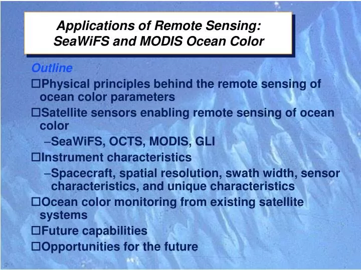
Applications of Remote Sensing: SeaWiFS and MODIS Ocean Color. Outline Physical principles behind the remote sensing of ocean color parameters Satellite sensors enabling remote sensing of ocean color SeaWiFS, OCTS, MODIS, GLI Instrument characteristics

E N D
Applications of Remote Sensing: SeaWiFS and MODIS Ocean Color Outline • Physical principles behind the remote sensing of ocean color parameters • Satellite sensors enabling remote sensing of ocean color • SeaWiFS, OCTS, MODIS, GLI • Instrument characteristics • Spacecraft, spatial resolution, swath width, sensor characteristics, and unique characteristics • Ocean color monitoring from existing satellite systems • Future capabilities • Opportunities for the future
Ocean Color Time Series Remote Sensing • “Course” spatial resolution (i.e., >1 km) but frequent temporal resolution (i.e., every other day) • Low marine biomass/high primary production • Marine primary production poorly understood • Single satellite with wide field of view (i.e.,CZCS and SeaWiFS) • Highly variable atmospheric effects • Variable directional reflectance effects • Forming composite images is the key • Coastal Zone Color Scanner (1979-1986) • SeaWiFS (August 1997 › …) • MODIS (February 2000 › …)
Sea-viewing Wide Field of View Sensor Applications • Ocean Color Studies — all channels • Atmospheric Studies (clouds, aerosols) — all channels • Land Vegetation Index — all channels • Cryosphere Studies — all channels Objectives • To determine the spatial and temporal distributions of phytoplankton blooms, along with the magnitude and variability of primary production by marine phytoplankton on a global scale • To quantify the ocean’s role in the global carbon cycle and other biogeochemical cycles • To identify and quantify the relationships between ocean physics and large-scale patterns of productivity
SeaWiFS Mission Characteristics and Sensor Accuracy • Radiative Accuracy: <5% absolute each band • Relative Precision: <1% linearity • Between Band <5% relative band-to-bandPrecision: (over 0.5 - 0.9 full scale) • Polarization: <2% sensitivity (all angles) • Nadir Resolution: 1.1 km LAC, 4.5 km GAC • Orbit Type: Sun synchronous at 750 km • Equator Crossing: Noon ± 20 minutes descending • Saturation Recovery: <10 samples • Swath Width 2,801 km LAC(at equator) 1,502 km GAC • Scan Plane Tilt +20°, 0°, -20° • Digitization: 10 bits
OrbView-2 Satellite and SeaWiFS Scanning Geometry Launched August 1, 1997
NASA, OrbView-2 launched August 1997 descending polar orbit of 705 km, noon crossing time Sensor Characteristics eight spectral bands, from 412 to 865 nm daily global coverage scan angle of ±58.3°; scan swath of 2800 km ±20° tilt to avoid sun glint resolution of 1.13 km (with optional 4.5 km) at nadir solar and lunar maneuvers for calibration polarization sensitivity ≤ 1% Sea-viewing Wide Field-of-view Sensor (SeaWiFS)
Rayleigh Scattering Coefficients for the Eight SeaWiFS Channels
OrbView-2 Launch Sequence and Satellite with Solar Panels Deployed
Ca chlorophyll-a Cb chlorophyll-b Cc chlorophyll-c Cps photosynthetic carotenoids Cpp photoprotectant carotenoids Ctp total pigment concentration, a sum of all the other parameters Simulated Pigment Absorption and Chlorophyll-a versus Total Pigments
Simulated Pigment Absorption and Chlorophyll-a versus Total Pigments
Correlation of AVHRR Sea Surface Temperature and Chlorophyll-a Concentration July 1998
SeaWiFS Captures El Niño/La Niña Transitions in the Equatorial Pacific Ocean: Chlorophyll-a Concentration Land: Normalized Difference Vegetation Index
Coccolithophore Bloom in the Bering Sea April 25, 1998
Chlorophyll and SeaWiFS-derived NDVI September-November 1997
Chlorophyll and SeaWiFS-derived NDVI December 1997 - February 1998
Moderate Resolution Imaging Spectroradiometer (MODIS) on Terra Terra MODIS
MODIS Ocean Color/Phytoplankton Bands BandBandwidthSpectral RadianceRequired SNR 8 405 - 420 44.9 880 9 438 - 448 41.9 838 10 483 - 493 32.1 802 11 526 - 536 27.9 754 12 546 - 556 21.0 750 13 662 - 672 9.5 910 14 673 - 683 8.7 1087 15 743 - 753 10.2 586 16 862 - 877 6.2 516