Download
1 / 23
230 likes | 391 Views
JP1.29 EFFECTIVE USE OF REGIONAL ENSEMBLE DATA IN FORECASTING. By Richard H. Grumm National Weather Service State College PA 16803 and Robert Hart The Pennsylvania State University. Introduction. Two winter storms one well forecast one poorly forecast Why we need ensembles

E N D
JP1.29 EFFECTIVE USE OF REGIONAL ENSEMBLE DATA IN FORECASTING By Richard H. Grumm National Weather Service State College PA 16803 and Robert Hart The Pennsylvania State University
Introduction • Two winter storms • one well forecast • one poorly forecast • Why we need ensembles • one model many potential initial states! • Physics differences and potential impact on forecasts • avoid model of the day problem: pick a single solution which may or may not be correct (binary YES/NO) • deal with uncertainty and probabilities • Mesoscale ensembles help to deal with: • Uncertainties in data • Uncertainties in data verse resolution • Uncertainties in physics require display strategies • Need to consider how to display these data
Ensemble Strategies • Lagged Average Forecasts (LAF) • dProg/dt feature in AWIPS • simple uses 1 model and different runs • last member considered most skillful • Single model with perturbed members • all members should be of similar skill • all initialized at same time (better than LAF) • NCEP MRF-ENS system • Ensemble of many models • NCEP SREF System • Eta in SREF not current operational Eta • RSM in SREF physics are older than AVN/MRF • “super ensemble”
Envelope of solutions at single time Solution Forecasts Initialized at most recent data time Forecast Length Ensembles with different initial conditions
Case 1: 3-4 Dec 2000 Winter Storm Case • 22-km Eta had more QPF and farther west then operational AVN • There was a trend in the models (dProg/dt) • SREF data • showed uncertainty • Eta members clustered different than RSM members • allowed forecasters to view uncertainty • provided visual cues on high and low probability areas for Winter Storm Warning (WSW) products.
0000 UTC 2 December • Cyclone Track difference • 0.20 QPF forecasts • advisory snow over most of region • 0.50 QPF forecasts • warning snow over most of region • T850 • will it snow or rain?
1200 UTC 2 December • Cyclone Track difference • 0.20 QPF forecasts • advisory snow over most of region • 0.50 QPF forecasts • warning snow over most of region • T850 • will it snow or rain?
3-4 Dec 2000 summary • SREFs • provided useful information • were better than any single model when considering high probability outcomes • QPF • good at low amounts • not so good high amounts (>0.70) • Thermal character • good for probabilities snow/ZR/Rain • Not a fluke as SREF’s did very well on 30 Dec 2000 Storm
SREFs Ain’t Perfect • Recent event 06-07 January failure • in defense AVN/Eta were slow to adjust • SREF never did adjust • heavy snow low probability in PA • Out of the “envelope solution” • the system is not perfect • NCEP aware and working on problems • Never rely on SREF alone • blend more skillful AVN/Eta • use AVN/Eta to evaluate strength of system • ensemble consensus waters down anomalous aspects of systems.
First cut at the snowfallcourtesy of the Pennsylvania State University
Figure 2: Eta 00-hour forecast of MSLP and 700 hPa heights initialized at 0000 UTC 7 January 2002. Anomalies are shown in the color bar to the left. Figure 3: As in Figure 2 except 850 hPa winds valid at 0000 UTC 7 January 2002. What verifiedan anomalously deep cyclone and easterly jet
Figure 7: 2100 UTC 5 January 2002 SREF and operational Eta (BLUE) and AVN (RED) initialized at 0000 UTC 6 January 2002. Forecast show probability and consensus and spaghetti plots Figure 8: SREF and operational Eta and AVN MSLP forecasts. Eta is in Blue and AVN is in red. Forecasts from 2100 UTC 5 January SREF and 0000 UTC Eta and AVN. SREF-enhanced by Eta/AVN
Figure 9. As in Figure 7 except 0900 UTC SREF and 1200 UTC 6 January 2002 operational Eta and AVN forecasts of 0.40 and 0.60 inches of QPF for the 24-hour period ending 09Z 07 January 2002. Note Eta is blue and AVN is red. More QPF
SREF Conclusions • show great promise on some events • did well 3-4 Dec and 30 Dec 2000 indicating • areas of heavy snow • areas rain/snow • cyclone track, out performing 22-km Eta • did poorly 6-7 Jan 2002 • QPF too far east, not enough to west • model divergence smoothed out how anomalous system was • operational models caught on and showed potential faster • SREF system is not perfect (but getting better!) • RSM is older code will be updated Spring 02 • Eta is older version than 12km Eta to be updated Jan 02
Consider this • NCEP SREF data • a valuable forecast tool and resource • can be used to exploit all visual concepts with ensembles • Consider this:One detailed mesoscale model (the model of the day) will allow the user to make highly specific and detailed inaccurate forecast.