Download

1 / 34
340 likes | 443 Views
Width Minimization i n the Single-Electron Transistor Synthesis. Speaker: Chian Wei Liu Advisor: Dr. Chun-Yao Wang 2013/07/28. OUTLINE. Introduction Motivation Width minimization approach Experimental result Future work. Introduction. current detector.

E N D
Width Minimization in the Single-Electron Transistor Synthesis Speaker: Chian Wei Liu Advisor: Dr. Chun-Yao Wang 2013/07/28
OUTLINE • Introduction • Motivation • Width minimization approach • Experimental result • Future work
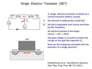
Introduction current detector • SET: Single-Electron Transistor • An SET array can be presented as a graph composed of hexagons 1
Example • An example of a XOR b: • ab’+ba’ active high a active low short a open b b • All sloping edges areconfigurable • short, open, active (high or low) • Active edges at the same row are controlled by a single variable
Mapping Constraint • Granularity constraint • Two edges are configured simultaneously • The combination of n.left and n.right, (n.left,n.right), must be one of (high, low), (low, high), (short, short),and (open, open), where n is a node in the SET array. • Fabric constraint • (high, low) and (low, high) cannot simultaneously appear in a row
OUTLINE • Introduction • Motivation • Width minimization approach • Experimental result • Future work
Motivation 0 0 • The previous work focuses on reducing the number of hexagons in SET arrays while the area is more related to the width. 1 1 2 2 3 3 4 4 P0: --001 P1: --110 P0: -0101 P1: -1010 1 1 -3 -2 -1 0 1 2 3 -3 -2 -1 0 1 2 3
Problem Formulation • Given: • An boolean circuit. • Objective: • Configuring the boolean circuit into SET arrays result in smaller width.
OUTLINE • Introduction • Motivation • Width minimization approach • Experimental result • Future work
Key Idea • In the previous work, for simplification, they allow only one of (high, low) and (low, high) to appear in an SET array • For width minimization, we allow both (high, low) and (low, high) to appear in an SET array • Architecture relaxation • More Branch-then-Share can be used • Limiting expansion of the SET array
Architecture Relaxation • Branch-then-Share • A good share relationship between product terms • They branch in one row and merge in the succeeding row such that the remaining edges are all shared.
Architecture Relaxation • More Branch-then-Share can be used Architecture requirement Type 1:(high,low) (high,low)or (low, high) (low, high) • (1,0)(0,1) (1,-)(0,1) (1,0)(0,-) (1,-)(0,-) Type 2:(high,low) (low,high) or (low, high) (high, low) • (1,1)(0,0) (1,-)(0,0) (1,1)(0,-) (1,-)(0,-)
Architecture Relaxation • Limiting expansion of the SET array 0 0 1 1 2 2 3 3 4 4 1 1 -4 -3 -2 -1 0 1 -2 -1 0 1
Width Minimization Approach • Product terms computation from Threshold Networks • Variables reordering • Architecture relaxation • Product terms reordering
Product Terms Computation from Threshold Networks • A threshold network is a network composed of linear threshold gates (LTG). • Computing product terms from LTG networks • Swapping the symmetric inputs
Computing product terms from LTG networks • Assuming the weights are integers • The weights of an LTG are positive • Computing its disjoint product terms from the primary output (PO) towards the primary inputs (PIs)
Swapping the symmetric inputs • For the LTG in the PO, only recording the locations of “–” from its onset • For other LTGs, recording the locations of a don’t its onset and offset • Swapping these symmetric inputs so that each don’t care “–” corresponds to a larger faningate
Variables Reordering • Front-end column determination • Moving the variables which have the same bit value among all product terms to the front-end of the variable ordering. • Remaining column reordering to determine • Determining the ordering according to quantity of bit value, 0, 1, -, in each variables among all product terms. • Avoiding destroying the Branch-then-Share.
Variables Reordering • Remaining column reordering to determine
Architecture Relaxation • Branch-then-Share Collection • Architecture determination
Branch-then-Share Collection P1: 110100 P2: 1100-- P3: 1111-- P4: 111000 P5: 11101- P1: 110100 P2: 1100-- P3: 1111-- P4: 111000 P5: 11101- P1: 110100 P2: 1100-- P3: 1111-- P4: 111000 P5: 11101- NBS: 1 NBS: 1 NBS: 2 NBS: 1 and 1 NBS: 2 Type conflict Group conflict (a) collect all the Branch-then-Shares (b) Select maximum of usable Branch-then-Shares (c) eliminate conflicting Branch-then-Shares
Architecture Determination • The first row is always configured as (high,low) • When there is a Branch-and-share, determine the row structure to meet the Branch-and-share requirement • Other row structures are determined as the previous row structure if over half of variables changes their value • Otherwise, inverse the row structure
Architecture Determination (1)(2)(3)(4)(5)(6) P1:110100 P2:1100-- P3:1111-- P4:111000 P5:11101- Row’s architecture (1) High, Low (2) Low, High (3) High, Low (4) Low, High (5) Low, High (6) High, Low
Product terms reordering • Grouping product terms • Scanning all the product terms from the first variable to the last one until at least one of product terms have different bit values on the variable. • Predict don’t care bits and EBL (expansion and branch level) According to the bit values and architectures. • Product term ordering determination • Determine the product term order by expansion level, share collection and group relation • Priority: share collection > group relation > expansion level
Product Terms Reordering (1)(2)(3)(4)(5)(6) P1:110100 P2:1100-- P3:1111-- P4:111000 P5:11101- Row’s architecture P1~P5 (1) High, Low (2) Low, High (3) High, Low (4) Low, High (5) Low, High (6) High, Low 111 110 P3~P5 1110 1111 P1 P2 110100 P1 110001 P2 111110 P3 111000 P4 111010 P5 P1: 4 P2: 3 P3: 3 P4: 5 P5: 4 P4 P5 P2->P3->P5->P4->P1 P3
Example-mapping result Previous work Width optimization approach P2:1100-- P3:1111-- P5:11101- P4:111000 P1:110100 Width=13 Width=9
A boolean circuit Overall flow Product terms computation LTG-based method BDD-based method Smaller product terms Branch-then-Share collection Collect all share types of Branch-the-Shares. Check conflicts. Select maximum share group and eliminate others conflicts. Variables reordering Move all-shared variables to the front. Reorder remaining variables according to the quantity of bit values in the variable among all the product terms. Architecture determination Configure the first row architecture as (high, low). Configure the following row architectures according to the share type and quantity of bit values switching. Product terms reordering Grouping the product terms. Predict the don’t care bit and EBL for product terms. Determine the ordering. Mapping process Set arrays
OUTLINE • Introduction • Motivation • Width minimization approach • Experimental result • Future work
OUTLINE • Introduction • Motivation • Width minimization approach • Experimental result • Future work
Future Work • Adjusting don’t care bits prediction