Download
1 / 38
440 likes | 1.17k Views
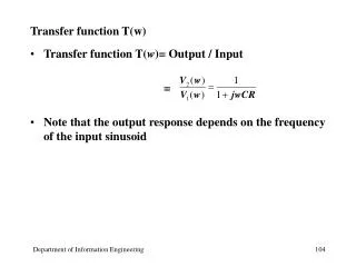
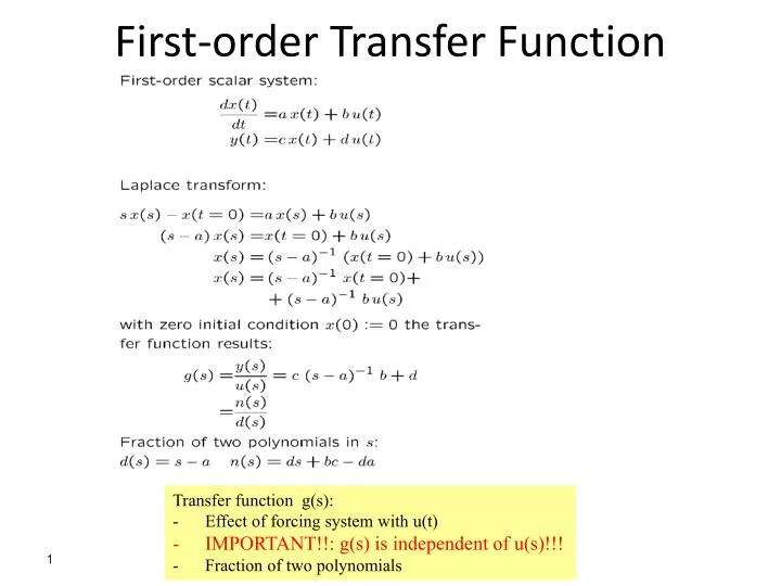
First-order Transfer Function. Transfer function g(s): Effect of forcing system with u(t) IMPORTANT!!: g(s) is independent of u(s)!!! Fraction of two polynomials. TexPoint fonts used in EMF. Read the TexPoint manual before you delete this box.: A A A A A A A A A.

E N D
First-order Transfer Function Transfer function g(s): • Effect of forcing system with u(t) • IMPORTANT!!: g(s) is independent of u(s)!!! • Fraction of two polynomials H Preisig 2006: Prosessregulering / S. Skogestad 2012 TexPoint fonts used in EMF. Read the TexPoint manual before you delete this box.: AAAAAAAAA
General Transfer Matrix The n roots(generallycomplex) ofthe polynomial d(s) arethe same as theeigenvaluesofthestatematrix A, and areknown as the «poles» ofthe system
Poles and zeros • What are transfer functions effect of forcing system • What is a forced system and why do we force a system • Transfer functions G(s) of linear, time-invariant networks of first-order systems are ratios of two polynomials in s (Laplace variable which relates to frequency) • Polynomials have rootsroot in denominator G(s) ”pole”root in numerator G(s) 0 ”zero” • Roots & dynamics • Numeratorrootsareresponsible for inverse or normal response • Denominatorrootsdeterminestability • Fast or slowdynamics H Preisig 2006: Prosessregulering
Dynamicstepresponseofsome systems TexPoint fonts used in EMF. Read the TexPoint manual before you delete this box.: AAAAAAAAAA
Step Response 3 2.5 2 1.5 Amplitude 1 0.5 0 0 5 10 15 20 25 30 35 40 Time (seconds) s=tf('s') g1 = 2/(10*s+1) step(g1,50) axis([0 40 -0.2 3]) First-order system (k=2, ¿=10) /) y u g1 y(t) 63% u(t) M
Initial and final values for stepresponse • Considerresponse y(t) to stepofmagnitudeM in input • Transfer function g(s) • Deviation variables for y(t) and u(t)
Step Response 3 2.5 2 1.5 Amplitude 1 0.5 0 0 5 10 15 20 25 30 35 40 Time (seconds) s=tf('s') g1 = 2/(10*s+1) step(g1,50) axis([0 40 -0.2 3]) First-order system (k=2, ¿=10) /) y u g1 y(t) 63% u(t) M
Step Response 3 2.5 2 1.5 Amplitude 1 0.5 0 0 5 10 15 20 25 30 35 40 Time (seconds) Larger time constant (¿=12) givesslowerdynamics s=tf('s') g1 = 2/(10*s+1), step(g1,50) axis([0 40 -0.2 3]); hold on, g2 = 2/(12*s+1), step(g2,50) g1 g2
Larger steady-stategain (k=2.2) s=tf('s') g1 = 2/(10*s+1), step(g1,50) axis([0 40 -0.2 3]); hold on, g2 = 2/(12*s+1), step(g2,50) g3 = 2.2/(10*s+1), step(g3,50) g3 g1 g2
Step Response 3 2.5 2 1.5 Amplitude 1 0.5 0 0 5 10 15 20 25 30 35 40 Time (seconds) Integrating system (g4=0.2/s) g1 & g4: Same initial response (slope = 0.2=k/¿) s=tf('s') g1 = 2/(10*s+1), step(g1,50) axis([0 40 -0.2 3]); hold on, g2 = 2/(12*s+1), step(g2,50) g3 = 2.2/(10*s+1), step(g3,50) g4 = 2/(10*s+0), step(g4,50) g4=0.2/s g3 g1 g2
Integrating system, g(s)=k’/s • Special case of first-order system with ¿=1and k=1 but slope k’=k/¿ is finite • g(s)=k/(¿s+1) = k/(¿ s) = k’/s • Step response (u=M): y(t)/M = k’t
Step Response 3 2.5 2 1.5 Amplitude 1 0.5 0 0 5 10 15 20 25 30 35 40 Time (seconds) Integrating system with time delay (g5) s=tf('s') g1 = 2/(10*s+1), step(g1,50) axis([0 40 -0.2 3]); hold on, g2 = 2/(12*s+1), step(g2,50) g3 = 2.2/(10*s+1), step(g3,50) g4 = 2/(10*s+0), step(g4,50) g5 = 2*exp(-5*s)/(10*s), step (g5,50) g4 g5 g1
Step Response 3 2.5 2 1.5 Amplitude 1 0.5 0 0 5 10 15 20 25 30 35 40 Time (seconds) g1 = 2 -------- 20 s + 1 g2 = 2 ---- 20 s g3 = 2 -------- 20 s - 1 Unstable system (e.g., exothermicreactor): Signchange in denominator d(s) g2 g3 unstable Integrating system: onthe limit to unstable g1 stable Oops… Negative sign in d(s)… Unstable!
Step Response 3 2.5 System: g3 Time (seconds): 21.9 2 Amplitude: 1.86 1.5 Amplitude 1 0.5 0 0 5 10 15 20 25 30 35 40 Time (seconds) «S-shaped» 2nd order responses (g2, g3, g4) made from two first-order systems in series g1 = 2/(10*s+1), step(g1,50) g2 = 2/[(10*s+1)*(10*s+1)], step(g2,50) g3 = 2/[(5*s+1)*(5*s+1)], step(g3,50) g4 = 2/[(10*s+1)*(2*s+1)], step(g4,50) g3 g4 g2 g1
Step Response 3 2.5 2 1.5 Amplitude 1 0.5 0 0 5 10 15 20 25 30 35 40 Time (seconds) g1 = 2/(10*s+1) g2 = 2/[(10*s+1)*(10*s+1)] 2nd order responses Special case(g2): ¿1=¿2=¿ 98% 86% 91% (96% at t=6¿) 63% 59% First-order Second-order with¿1=¿2=¿ g1 26% g2 t=4¿ t=¿ t=2¿
Step Response 3 2.5 2 1.5 Amplitude 1 0.5 0 0 5 10 15 20 25 30 35 40 Time (seconds) g1 = 2/(2*s+1), step(g1,50) g2 = 2/(2*s+1)^2, step(g2,50) g3 = 2/(2*s+1)^3, step(g3,50) g4 = 2/(2*s+1)^4, step(g4,50) g5 = 2/(2*s+1)^5, step(g5,50) g6 = 2/(2*s+1)^6, step(g6,50) g7 = 2/(2*s+1)^7, step(g7,50) n’th order responses: From n identical first-order systems in series g1 g7
General 2nd order system Roots (poles, eigenvalues): Chapter 5 Special case: Two first-order in series (overdamped, ³¸ 1):
Underdamped (Oscillating) second-order systems (³<1) • Corresponds to complex poles • Process systems: • Oscillationsareusuallycaused by (too) aggressive control • Example 1: P-controlof second-order process, k/(¿1 s+1)(¿2 s+1) • Oscillates (³<1) ifKck is large (seeexercise) • Example 2: PI-controlofintegratingprocess, k’/s • Needcontrol to stabilize • Oscillates (³<1) ifKck’ is small (seederivation SIMC PID-rules)
Step Response 1.4 1.2 1 0.8 Amplitude 0.6 0.4 0.2 0 0 2 4 6 8 10 12 Time (seconds) s=tf('s') zeta=0.5, tau=1 g = 1/[(tau*s)^2 + 2*tau*zeta*s + 1] step(g) g = 1 ----------- s^2 + s + 1 >> pole(g) ans = -0.5000 + 0.8660i -0.5000 - 0.8660i
Chapter 5 =a/b =c/a
Zeros Zeros • g(s) = n(s)/d(s) • Zeros: rootsofnumerator polynomial, n(s)=0 • Example, g1(s)= (3s+1)/(10s+1)(s+1). Zero: s=-1/3 • Problem for controlif n(s) has coefficientwith different signs (positive zeros in the right half plane (RHP). Give inverse response. • Example, g2(s)= (-3s+1)/(10s+1)(s+1). Zero: s=1/3 Oops… Negative sign in n(s)… Inverse response!
Zeros Step Response 2.5 2 1.5 Amplitude 1 0.5 0 0 5 10 15 20 25 30 35 40 Time (seconds) Zeros • Zeros arecommon in practise • Occurwhenthereareseveral «paths» to the output. • Example 1. • Example 2 • Example 3 g1(s) u y All coefficients positive: LHP zero g2(s) Signchange: RHP zero ) Inverse response 3 1 2 Note; Overshootsince 11.3>10
Zeros Step Response 2.5 2 1.5 1 0.5 0 0 5 10 15 20 25 30 35 40 Time (seconds) 2 RHP-zero with «time constant» -0.59: Similar to delayof 0.59.
Zeros Step Response 3 2.5 2 1.5 Amplitude 1 0.5 0 -0.5 0 5 10 15 20 25 30 35 40 Time (seconds) g1 = 2*(3*s+1)/[(10*s+1)*(s+1)], step(g1,50) g0 = 2/[(10*s+1)*(s+1)], step(g0,50) g2 = 2*(-3*s+1)/[(10*s+1)*(s+1)], step(g2,50) g1: LHP zero g0: No zero g2: Signchange for coeffcients in n(s) (RHP zero): Inverse response
Zeros Step Response 3 2.5 2 1.5 Amplitude 1 0.5 0 -0.5 -1 0 5 10 15 20 25 30 35 40 Time (seconds) Another Inverse responseexample (RHP zero: «competingeffectswhereslowwins»). Physicalexample: Increase hot water flowwhen water heater is onmax. u = qh, y = T • s=tf(‘s’) • g1 = 1 • g2 = 2/(10*s+1) • g=g1-g2 • ans= • 10 s - 1 • --------- • 10 s + 1 g = g1 - g2,
Zeros Step Response 3 2.5 2 1.5 Amplitude 1 0.5 0 -0.5 -1 0 5 10 15 20 25 30 35 40 Time (seconds) Anotherexample LHP zero: Note noovershoothere (effects in same direction) g = g1 + g2 g1 = 1 g2 = 2/(10*s+1),
Zeros k1 : “slow” effect (¿1 > ¿2) k = k1+k2 Zero at z=1/¿a z1: RHP-zero (z1<0, ¿a<0) • Inverse response= Competingeffects(k’s oppsitesigns) whereslowwins(|k1|>|k2|) z2:Zero at origin (z2=0, ¿a!1) • Competingeffectwith same magnitude (k1=-k2) • Steady-stategain is zero z3: LHP-zero close to RHP (¿a> ¿1, approx) • Overshoot = Competingeffectswherefast wins z4:LHP-zero far from RHP (¿a< ¿1, approx) • No overshoot= Effects in same direction (k1and k2 same sign) Im(s) z = 1/¿a z1 z3 z4 z2 o o o o x 1/¿1 Re(s)
Summary poles and zeros • Poles p (=eigenvalues of A) • Determine speed of response • p in RHP: unstable (NEED control) • P complex: oscillating response • Zeros z • Determine shape of response • z in RHP: inverse response (BAD for control)
Step Response 1 0.8 0.6 0.4 0.2 Amplitude 0 -0.2 -0.4 -0.6 -0.8 -1 0 0.5 1 1.5 2 2.5 3 3.5 4 4.5 5 Time (seconds) Approximations of time delay s=tf('s') theta=1 g0=exp(-theta*s) % time delay. theta g1= - theta*s + 1 % RHP-zero, taua=theta g2= 1/(theta*s+1) % first order, tau=theta g3 = (-theta*s/2+1)/(theta*s/2+1) % Pade-approx h=1/(s+1) step(g0*h,g1*h,g2*h,g3*h) axis([0 5 -1 1.1]) 2 0 3 1
Skogestad Half Rule* * S. Skogestad, “Simple analytic rules for model reduction and PID controller design”, J.Proc.Control, Vol. 13, 291-309, 2003 (Also reprinted in MIC)
Example 1 Half rule
Original 2nd order 1st-order+delay (half rule)
Step Response 1 0.8 0.6 Amplitude 0.4 Step Response 0.4 0.35 0.2 0.3 0.25 0 0.2 Amplitude 0.15 0.1 -0.2 0 5 10 15 20 25 30 35 40 0.05 Time (seconds) 0 -0.05 0 0.5 1 1.5 2 2.5 3 3.5 4 4.5 5 Time (seconds) s=tf('s') g=(-0.1*s+1)/[(5*s+1)*(3*s+1)*(0.5*s+1)] g1 = exp(-2.1*s)/(6.5*s+1) g2 = exp(-0.35*s)/[(5*s+1)*(3.25*s+1)] step(g,g1,g2) Example 2
c c c c c c Approximation of LHP-zeros To make these rules more general (and not only applicable to the choice c=): Replace (time delay) by c (desired closed-loop response time). (6 places) τc = desiredclosed-loop time constant