Download
1 / 18
180 likes | 383 Views
Computer Simulation of the Head-Related Transfer Function. COMP 768 Project Presentation. Alok Meshram 12/11/2012. Goals. Implement a Sound Simulation method/system Use it to generate Head-Related Transfer Functions given head geometry Analyze the output. Sound Simulation: FDTD.

E N D
Computer Simulation of the Head-Related Transfer Function COMP 768 Project Presentation AlokMeshram 12/11/2012
Goals • Implement a Sound Simulation method/system • Use it to generate Head-Related Transfer Functions given head geometry • Analyze the output
Sound Simulation: FDTD • The Finite-Difference Time Domain method approximates derivatives using differences in adjacent function values: • Using this approximation, the Acoustic Wave Equation is reduced to update equations in time and space • The simulation is carried out over spaceand time by using these update equationson a “staggered grid”
Sound Simulation: FDTD • In FDTD simulations implemented this way, boundaries of the spatial domain act as rigid reflectors • Free-field simulations, such as the one required for this project, require the presence of Absorbing Boundary Conditions(ABCs), which “absorb” waves propagating outside the domain. • A popular ABC is the Perfectly Matched Layer(PML) • Another important problem FDTD simulations suffer from is numerical dispersion: different frequency components travel with different speeds • This can result in distortion in the simulation • This problem can be avoided to a certain extent by smaller spatial steps – resulting in more mesh points, requiring more computational power
Sound Simulation: FDTD • For this project, I began with implementing FDTD with PML • A simple implementation of PML was achieved using “stretched coordinates” • These coordinates have an absorption coefficient included as an imaginary component • The absorption coefficient was set to 0 in the interior of the domain • To implement PML, the coefficient is steadily increased after a certain distance from the boundaries of the domain
FDTD: Issues • When implemented this way, the simulation worked well if the domain consisted only of a single material with constant parameters • However, when another material was present in the domain, the simulation started having significant numerical error propagating from the boundary of the two materials • This error reduced when using a finer mesh, but that also increased computation time significantly • This and the dispersion errors mentioned previously were problematic for HRTF generation as the requirement was the generation of an impulse response from reflection due to a reflective surface (head)
Adaptive Rectangular Decomposition • Instead of FDTD, I used the Adaptive Rectangular Decomposition (ARD) based Sound Simulator developed by NikunjRaghuvanshiand others from the GAMMA group • The basic idea behind ARD is to decompose the spatial domain into rectangular domains, and use the known solution of the wave equation in a rectangular space in each of these domains • Since the spatial part of the solution in rectangular space is sinusoidal, the problem can be solved using Fast Fourier Transforms. Since FFTs are efficient, this increases efficiency: O(n logn) vs. O(n2) in time • Another important advantage is that ARD does not have numerical dispersion errors
An overview of ARD. The spatial domain is subdivided into rectangles, and the solution of the wave equation carried in each of them. Sound is propagated through one rectangle to another through interfaces.
HRTF Generation using ARD Simulator • For the head geometry, I used the 3D Mesh of the KEMAR mannequin obtained courtesy of Dr. YuviKahana of Institute of Sound and Vibration Research, University of Southampton, UK • The KEMAR mannequin has been used extensivelyin 3D Sound research, and comprehensive datasetsof measured HRTFs of the KEMAR head are available online • The head was placed in a cubic room of dimensions1.2m x 1.2m x 1.2m with PML at the boundary • A Gaussian impulse source was placed 1m away from the head at various azimuth and elevation combinations
HRTF Generation using ARD Simulation • The cells in the simulation mesh were cubes of size approx. 8 mm • This corresponded to a maximum reliable frequency of approx. 15 kHz • The Gaussian source had a center frequency of approx. 7.5 kHz • A single simulation took about 2 hrs. to complete for 400 time steps, and generated an output file containing pressure values at all cell locations for each time step • The pressure values from the ear locations were extracted from this output file, obtaining the Left and Right Head Related Impulse Responses (HRIRs) • These Impulse Responses were processed by a MATLAB script to obtain the HRTF, and to plot it against measured HRTFs for the same source location (measured HRTFs obtained from the CIPIC database from UC Davis)
Results Left ear HRTF, Azimuth = 0 degrees, Elevation = 0 degrees
Results Right ear HRTF, Azimuth = 0 degrees, Elevation = 0 degrees
Results Left ear HRTF, Azimuth = -45 degrees, Elevation = 45 degrees
Results Right ear HRTF, Azimuth = -45 degrees, Elevation = 45 degrees
Results Left ear HRTF, Azimuth = -45 degrees, Elevation = 0 degrees
Results Right ear HRTF, Azimuth = -45 degrees, Elevation = 0 degrees
Observations • The Simulated HRTFs are significantly different from the Measured HRTFs, though somewhat structurally similar • Features such as peaks and valleys in the 5kHz – 10kHz range are missing • The primary reason is the coarse mesh (8 mm). Accurate HRTF simulations using FDTD have used meshes with a 2mm cell size. • Another important factor that added error to the simulation is that the PML implementation in the simulator did not work correctly, resulting in reflections from the boundaries
Future Work • It was observed that increasing the maximum frequency of the simulation (hence decreasing the cell size) improved results, but reaches the process memory limit (2 GB) on Windows for ~19000 kHz (used for this report) • Bypassing this barrier will allow simulation with a finer mesh, which will produce more accurate results • Furthermore, if the problem with the PML (reflections) is fixed, the results will increase considerably in accuracy • Finally, the material for the head used for this report was “Rough concrete”, which corresponded to maximum reflection. A material closer to the head material could produce better results