Download
1 / 21
210 likes | 337 Views
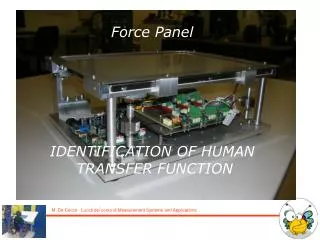
Force Panel IDENTIFICATION OF HUMAN TRANSFER FUNCTION. 2. Human Transfer Function. H( w ). Reference position (to be followed by the finger). Actual finger position. 3. Modelling.

E N D
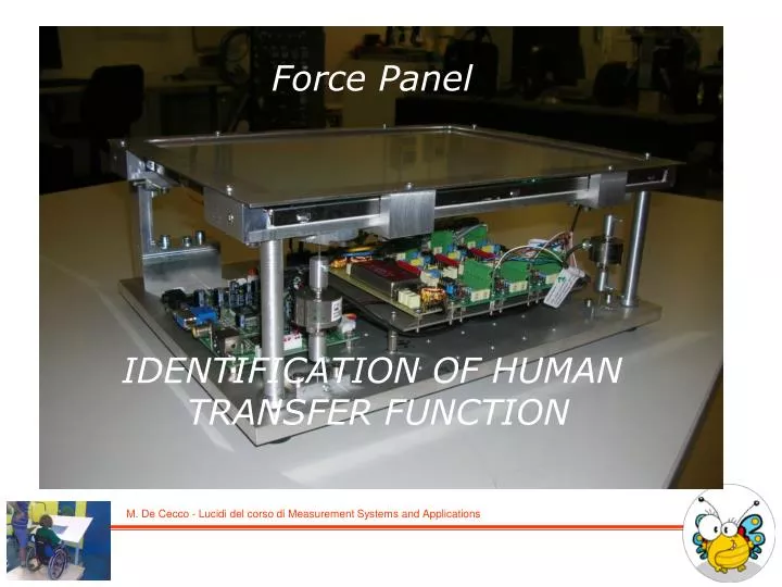
Force Panel IDENTIFICATION OF HUMAN TRANSFER FUNCTION
2 Human Transfer Function
H(w) Reference position (to be followed by the finger) Actual finger position 3 Modelling
Transfer functions have been used to model how human beings control several types of plants, for example the lane keeping task in automobiles (Kondo-like models) or route keeping in aircraft. A typical transfer function is the following: Where the gain K, the time delay and TN are parameters inherent of the human being (K is also task dependent), TI and TL are adaptive parameters that the subject changes (TL with mental workload) to adapt to the plant dynamics. Plöchl, Edelmann. Driver models in automobile dynamics application, Vehicle System Dynamics, Vol. 45, Nos. 7–8, pp 699–741 , July–August 2007 Simplified: 4 Modelling
Band-Limited Noise fc = 40 Hz Butterworth Lowpass Filter; 1st Order, ft = 0.1 Hz Input and output signals
The transfer function gives the possibility to directly simulate the user behaviour in interacting with any control panel. As an example: - to simulate the appearance of a button to press 100 mm far away from the hand position Noise PSD 100 100 Input: step function Output: simulated trajectory + noise (estimation of final position uncertainty) Model parameters: G = motion gain = time constant d = delay What if G is less than 1??? Why happens to be like that?? (typically 0.6) 6 button Human Transfer Function - simulating the task of pressing a button
7 Human Transfer Function - simulating a game interaction
Class work Identification in frequency
1th work in class: filter outliers due to low finger pressure Main steps – 1 filter outliers
2th work in class: filter the frequency ratio (that is too noisy to be used as it is) zoom Zoom of the zoom Main steps – 2 filter the FFT ratio
The considered HTF to find are: 1) 2) 3)
3th work in class: fit the modulus Main steps – 3 fit the modulus of the HTF
4th work in class: find the phase Main steps – 4 find the HTF delay (t)
% program to complete in class % [to do between square brackets] % so, find '[]' to localize where to write code (or functions) clear all close all; clc; %% Load DATA % [] % [copy the filename to elaborate and its directory] im = strcat('Dati/Segnale_5/fp_acq_03_04_20111004115703.txt'); [header, hh, dd] = readColData(im,8,7,1); tempo = dd(:,1); % time x = dd(:,2); % x finger position red by arduino [ bit ] y = dd(:,3); % y finger position red by arduino [ bit ] f1 = dd(:,4); % first load cell red by arduino [ bit ] f2 = dd(:,5); % second load cell red by arduino [ bit ] f3 = dd(:,6); % third load cell red by arduino [ bit ] x_segnale = dd(:,7); % x reference of the vertical line [ pixel ] x_touch = x * 1.19 - 108.55 ; % x finger position with respect to LCD (calibration) [ pixel ] ID = dd (:, 8 ) ; Class work
% extract time tempo = tempo - tempo(1) ; Tc = tempo(end) / length(tempo) ; tempo = 0 : (length(tempo) - 1) ; tempo = tempo * Tc ; % filter repeated data on the ARDUINO ID IIf = find( [ 1; diff(ID)] ) ; data_finger = x_touch( IIf ) ; % x finger position filtered data_input = x_segnale( IIf ) ; % x reference filtered tempo = tempo( IIf ) ; % time filtered tempo = tempo - tempo(1) ; figure, plot( tempo/1000, data_finger, 'b', tempo/1000, data_input, 'r' ) title('Reference and finger position'), grid on %% 1. Filtering outliers % [filtrare i salti dovuti a scarsa pressione del dito] meanF = mean (f1(IIf) + f2(IIf) + f3(IIf)) ; % mean of the load figure, plot( tempo/1000, data_finger, 'b', tempo/1000, (f1(IIf) + f2(IIf) + f3(IIf) - meanF) *10 + 300, 'r' ) title('Finger position and applied force'), grid on % [] soglia_Dx = 100 ; data_finger = FiltraOutliers_CELLE(data_finger, data_input, soglia_Dx) ; Class work
%% 2. Trasfer Function estimation data_input = data_input - mean(data_input) ; data_finger = data_finger - mean(data_finger) ; % FFT computation F_Iinput = fft(data_input) / length(data_input) ; F_Ooutput = fft(data_finger) / length(data_finger) ; % plot of the transform ratio Hs = F_Ooutput ./ F_Iinput ; Hs(1) = 1 ; % (to recover the fact that the mean values were just eliminated) ffTF = 1000 * ( 0:(length(data_input)-1) ) / tempo(end) ; % Frequency vector [Hz] figure, plot(ffTF, abs(F_Iinput), 'r'), hold on plot(ffTF, abs(F_Ooutput)) plot(ffTF, abs(Hs), 'c') legend('Input','Output','Hs') xlabel ('Frequency [Hz]') % [] % [to filter the experimental transfer function 'Hs' just obtained by FFT ratio] plotta = 1 ; Hs = Filtro_Hs( Hs, F_Iinput, F_Ooutput, ffTF, plotta ) ; Class work
%% just rename the variables: Iinput = data_input ; Ooutput = data_finger ; %% 3. FITTING modulus with lsqnonlin % [] % write a function 'FittingFrequenza' % par_ini = [0 2*pi*0.2 2*pi*0.1 2*pi*2] % solo primo ordine, 4 par par_ini = [0 2*pi*0.2 2*pi*0.1 0.7 2*pi*2] % anche secondo ordine, 5 par if length(par_ini) == 4 % 1th order par_ott = lsqnonlin(@(par) FittingFrequenza(par, Hs, ffTF, 0), par_ini, ... [0 0 0 0], [100 100 100 100]) ; elseif length(par_ini) == 5 % 2nd order par_ott = lsqnonlin(@(par) FittingFrequenza(par, Hs, ffTF, 0), par_ini, ... [0 0 0 0 0], [100 100 100 100 100]) ; % con [0 100 90 0 0] si fa 2d ordine end Class work
%__________________________________ % % 4. estimate the parameter delay %__________________________________ % [] % write a function simulink 'CompDinamica' that simulates the model without delay % use the function 'corr' to estimate the delay % 0. neglect the mean values Iinput = Iinput - mean(Iinput) ; Ooutput = Ooutput - mean(Ooutput) ; % 1. dynamical simulation without delay par = par_ott ; if length(par) == 4 % solo primi ordini sim('CompDinamica_1ord') elseif length(par) == 5 % secondo ordine sottosmorzato sim('CompDinamica_2ord') end Comp_Iinput = interp1(time, Comp_Iinput, tempo/1000)' ; Class work
% 2. correlation of the output with the simulated output (without delay) % [] % [use the function 'corr'] tau = 0 ; par_ott(1) = tau ; % plot results FittingFrequenza(par_ott, Hs, ffTF, 1) ; % !!!!!!!!!!!!!!!!!!!!!!!!! ModelloHTF(par_ott, ffTF, 1) ; %% SIMULATION OF A STEP INPUT WITH THE HTF par = par_ott ; if length(par) == 4 % 1th order sim('simulazione_1ord') elseif length(par) == 5 % 2nd order sim('simulazione_2ord') end figure, plot(time, step, time, step_out), title('Step input simulation') Class work