Download
1 / 72
790 likes | 1.11k Views
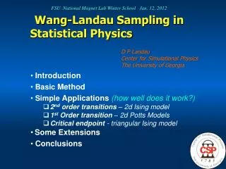
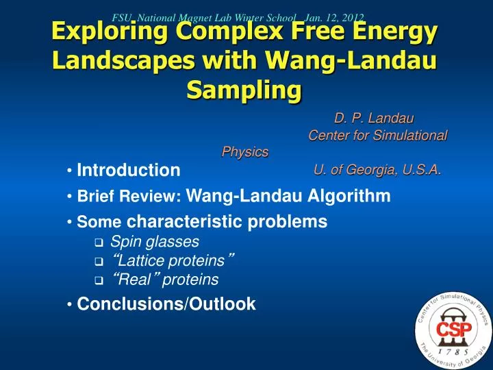
FSU National Magnet Lab Winter School Jan. 12, 2012. Exploring Complex Free Energy Landscapes with Wang-Landau Sampling D. P. Landau Center for Simulational Physics U. of Georgia, U.S.A . Introduction Brief Review: Wang-Landau Algorithm Some characteristic problems

E N D
FSU National Magnet Lab Winter School Jan. 12, 2012 Exploring Complex Free Energy Landscapes with Wang-Landau SamplingD. P. Landau Center for Simulational Physics U. of Georgia, U.S.A. • Introduction • Brief Review: Wang-Landau Algorithm • Some characteristic problems • Spin glasses • “Lattice proteins” • “Real” proteins • Conclusions/Outlook
Many systems in nature have complex or “rough” free energy landscapes in which there are many maxima and minima that may have widely spaced values of relevant thermodynamic parameters. At “low” temperature, transitions between minima become veryinfrequent Almost all models for such systems are impossible to treat analytically! Background and motivation
Simulation NATURE Experiment Theory
Reminder from Statistical Mechanics ThePartition functioncontains all thermodynamic information: Metropolis Monte Carlo approach: sample states via a random walk in probability space The “fruit fly” of statistical physics: The Ising model For a system of N spins have 2N states!
Single spin-flip sampling for the Ising model Produce the nth state from the mth state … relative probability is Pn /Pm need only the energy difference,i.e. E=(En-Em)between the states Any transition rate that satisfiesdetailed balanceisacceptable, usually the Metropolis form(Metropolis et al, 1953).W(mn) = o-1 exp (-E/kBT), E > 0= o-1 , E < 0 where ois the time required to attempt a spin-flip.
MC Problems and Challenges Statics:Monte Carlo methods are valuable, but near Tc critical slowing downfor2nd ordertransitions metastabilityfor1st ordertransitions and for systems with complex energy landscapes Try to reduce characteristic time scales or circumvent them
Center for Stimulational PhysicsCenter for Simulated Physics
Center for Stimulational PhysicsCenter for Simulated Physics
The “Random Walk in Energy Space with a Flat Histogram” method or “Wang-Landau sampling” Wang and Landau, PRL (2001)
Wang-Landau sampling Random Walk in Energy Space with a Flat Histogram Estimate the density of statesg(E) directly by performing a random walk in energy space: 1.Set g(E)=1; choose a modification factor(e.g. f0=e1) 2. Randomly flip a spin with probability: 3.Setg(Ei) g(Ei)*f, H(E)H(E)+1 4. Continue until the histogram is “flat” decreasef, e.g. fi+1=f 1/25. Repeat steps 2 - 4 untilf= fmin~ exp(10-8)6. Calculate properties using final density of states g(E)
Density of States for the 2-dim Ising model Compare exact results with data from random walks in energy space:LL lattices with periodic boundaries = relative error( exact solution is known for L 64 )
Free Energy of the 2-dim Ising Model = relative error
Applications to “Complex” Systems • Spin glasses • “Lattice proteins” • “Real” proteins
A Magnetic System with Complex “Order” At Tc (if it exists) a spin glass state forms get a “rough” energy landscape where multiple minima are separated by high energy barriers
A Magnetic System with Complex “Order” At Tc (if it exists) a spin glass state forms get a “rough” energy landscape where multiple minima are separated by high energy barriers This is just an Ising model with random interactions
A Magnetic System with Complex “Order” At Tc (if it exists) a spin glass state forms get a “rough” energy landscape where multiple minima are separated by high energy barriers Define an Order Parameter ‘q’ Overlap of a configuration with a groundstate . . . but must also take the configurational average over different bond distributions Extend random walk two-dimensional parameter space
Distribution of States: LxLxL EA Spin Glass L=6 . . . For larger L, P(q,T) becomes even more complex!
Distribution of States: LxLxL EA Spin Glass . . . For larger L, P(q,T) becomes even more complex!
Distribution of States: LxLxL EA Spin Glass Warning ! Dayal et al. (PRL, 2004) showed that for local updates, the tunneling time has exponential scaling -> very long tunneling times between some states for some big systems . . . For larger L, P(q,T) becomes even more complex!
Groundstate Properties of the 3-d EA Spin Glass Entopy and energy for the LLL simple cubic lattice Wang-Landau sampling Multicanonical sampling* L S0 E0 S0 E0 4 0.075+0.027 -1.734+0.006 0.0724+0.0047 -1.7403+0.0114 6 0.061+0.025 -1.767+0.024 0.0489+0.0049 -1.7741+0.0074 8 0.049+0.007 -1.779+0.016 0.0459+0.0030 -1.7822+0.0081 12 0.053+0.001 -1.780+0.012 0.0491+0.0023 -1.7843+0.0030 16 0.058+0.004 -1.776+0.004 20 0.056+0.003 -1.774+0.004 * Berg, Celik, and Hansmann (1993)
Applications to “Complex” Systems • Spin glasses • “Lattice proteins” • “Real” proteins
A Biological “Grand Challenge”: Protein Folding Real proteins are long polymers with side chains of different types and complicated interactions simplify . . . but how much?
Introduction A “Biologically inspired” problem The HP model of protein folding Amino acid = “bead” Hydrophobic (H) Polar (P) Protein sequence = “HPHPPHHPHPP…” Protein conformation = “self-avoiding walk” on a lattice, e.g. square (2D), cubic (3D)
A “Biologically inspired” problem The HP model of protein folding Amino acid = “bead” x Hydrophobic (H) Polar (P) x Protein sequence = “HPHPPHHPHPP…” x Protein conformation = “self-avoiding walk” on a lattice, e.g. square (2D), cubic (3D) Nearest-neighbor interactions between non-covalently bound neighbors Compact hydrophobic core / polar (hydrophilic) shell EHH = -1, EHP = 0, EPP = 0 (Dill, Biochemistry 1985; Lau, Dill, Macromolecules 1989)
A “Biologically inspired” problem The HP model of protein folding Amino acid = “bead” x Hydrophobic (H) Polar (P) x Protein sequence = “HPHPPHHPHPP…” x Protein conformation = “self-avoiding walk” on a lattice, e.g. square (2D), cubic (3D) Sequences are chosen to mimic real proteins Nearest-neighbor interactions between non-covalently bound neighbors Compact hydrophobic core / polar (hydrophilic) shell EHH = -1, EHP = 0, EPP = 0 (Dill, Biochemistry 1985; Lau, Dill, Macromolecules 1989)
Wang-Landau sampling with pull moves The importance of move sets Local moves: Non-local moves: End flip (1 bond) Pivot move Kink flip (2 bonds) Crankshaft (3 bonds) ergodic … but inefficient for dense conformations high rejection probability non-ergodic
3 2 3 2 Wang-Landau sampling with pull moves Pull moves 5 4 7 6 8 9 1 multi-bead move (Completes internally) multi-bead move (Pulls until the end of the sequence) (Lesh et al., 2003)
Wang-Landau sampling with pull moves Pull moves Extensible to any dimension Ergodic (complete) Reversible • n(A B) = n(B A) (detailed balance!) 7 6 5 8 4 3 No time-consuming self-avoidance test required 9 1 2 Good balance: local non-local “Close-fitting” High acceptance ratio Ideal for Wang-Landau sampling
Wang-Landau sampling of the HP model • With pull moves
“Cut and join” moves Initial HP configuration (Deutsch, J. Chem. Phys. 1997)
“Cut and join” moves (Deutsch, J. Chem. Phys. 1997)
“Cut and join” moves Note: For the HP model, the sequence of H’s and P’s must be maintained (Deutsch, J. Chem. Phys. 1997)
Wang-Landau sampling of the HP Model 64mer in 2 dimensions (square lattice) Seq2D64 Ground state search • Core directed chain-growth(Beutler, Dill 1996) • PERM (Bastolla et al. 1998) Ground state (E =-42) Density of states • Multi-self-overlap ensemble (MSOE)(Chikenji et al. 1999) • Equi-energy sampling (EES)(Kou et al. 2006)
Wang-Landau sampling of the HP Model 64mer in 2 dimensions (square lattice) Seq2D64 Ground state search • Core directed chain-growth(Beutler, Dill 1996) • PERM (Bastolla et al. 1998) Ground state (E =-42) Density of states • Multi-self-overlap ensemble (MSOE)(Chikenji et al. 1999) • Equi-energy sampling (EES)(Kou et al. 2006) Hydrophobic core
Wang-Landau sampling of the HP Model 64mer in 2 dimensions (square lattice) Seq2D64 Ground state search • Core directed chain-growth(Beutler, Dill 1996) • PERM (Bastolla et al. 1998) Ground state (E =-42) Density of states • Multi-self-overlap ensemble (MSOE)(Chikenji et al. 1999) • Equi-energy sampling (EES)(Kou et al. 2006) Hydrophilic surface
Benchmark sequences: A performance analysis A “Biologically inspired” problem The HP Model of Protein Folding Seq2D64
The HP model of protein folding 64er in 2 dimensions (square lattice) Seq2D64 Ground state (E = -42) 1st excited state (E = -41)** **highly degenerate
Wang-Landau Sampling of the HP model 103mer in 3 dimensions (simple cubic lattice) Seq3D103 Ground state (E = -58) Ground state search • Fragment regrowth MC(Zhang, Kou et al. 2007) Density of states • Multicanonical chain-growth (MCCG)(Bachmann, Janke 2003 / 2004)
The HP model of protein folding Seq3D103: Thermodynamic properties Two-step folding process Density of states Specific heat 5 runs 80hCPU / run
The HP model of protein folding 103mer in 3 dimensions (cubic lattice) Ground state (E = -58) 1st excited state (E = -57)
Now introduce an attractive surface: The HP model of protein folding EHH = H–H bond interaction energy ΕSH = H–surface interaction energy ESP= P–surface interaction energy We have studied ESH=ESP, but other surfaces can be easily simulated!
36mer in 3 dimensions (cubic lattice) with a surface The HP model of protein folding ESH=ESP=EHH/12
36mer in 3 dimensions (cubic lattice) with a surface The HP model of protein folding ESH=ESP=EHH/12
36mer in 3 dimensions (cubic lattice) with a surface The HP model of protein folding ESH= ESP= EHH/12
36mer in 3 dimensions (cubic lattice) with a surface The HP model of protein folding 2 ×4 ×2 hydrophobic core ESH= ESP= EHH/12
36mer in 3 dimensions (cubic lattice) with a surface The HP model of protein folding ESH= ESP= EHH/12
36mer in 3 dimensions (cubic lattice) with a surface The HP model of protein folding ESH= ESP= EHH/12