Download
1 / 34
340 likes | 497 Views
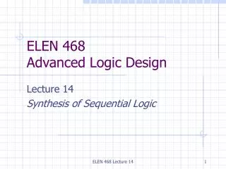
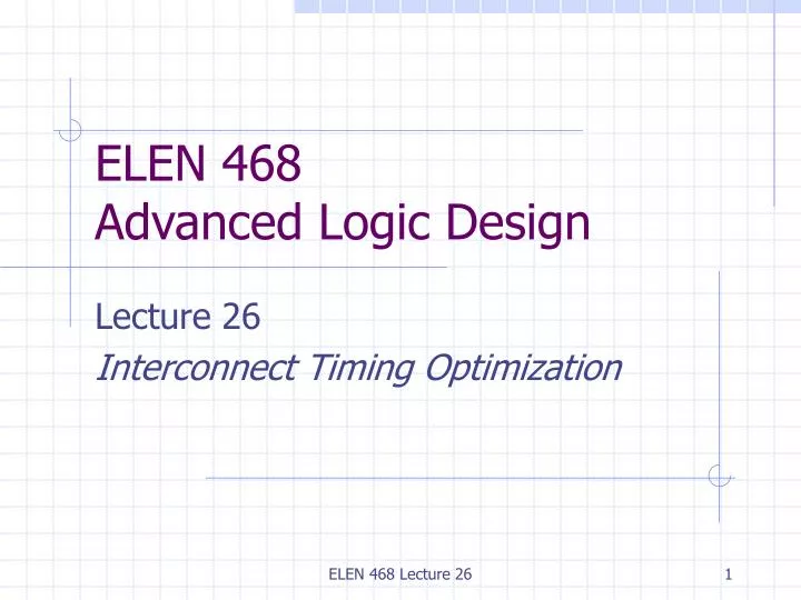
ELEN 468 Advanced Logic Design. Lecture 26 Interconnect Timing Optimization . x/2. x/2. R. C. rx/2. R. rx/2. cx/4. cx/4. cx/4. cx/4. C. ∆t. x. Buffers Reduce Wire Delay. t_unbuf = R( cx + C ) + rx( cx/2 + C ) t_buf = 2R( cx/2 + C ) + rx( cx/4 + C ) + t b

E N D
ELEN 468Advanced Logic Design Lecture 26 Interconnect Timing Optimization ELEN 468 Lecture 26
x/2 x/2 R C rx/2 R rx/2 cx/4 cx/4 cx/4 cx/4 C ∆t x Buffers Reduce Wire Delay t_unbuf = R( cx + C ) + rx( cx/2 + C ) t_buf = 2R( cx/2 + C) + rx( cx/4 + C) + tb t_buf – t_unbuf = RC + tb– rcx2/4 ELEN 468 Lecture 26
Buffers Improve Slack RAT = 300 Delay = 350 Slack = -50 slackmin = -50 RAT = 700 Delay = 600 Slack = 100 RAT = Required Arrival Time Slack = RAT - Delay RAT = 300 Delay = 250 Slack = 50 Decouple capacitive load from critical path slackmin = 50 RAT = 700 Delay = 400 Slack = 300 ELEN 468 Lecture 26
Problem Formulation • Given • A routing tree • RAT at each sink • A buffer type • RC parameters • Candidate buffer locations • Find buffer insertion solution such that the slackmin is maximized ELEN 468 Lecture 26
Candidate Buffering Solutions ELEN 468 Lecture 26
vi is a sink ciis sink capacitance vis an internal node Candidate Solution Characteristics • Each candidate solution is associated with • vi: a node • ci: downstream capacitance • qi: RAT ELEN 468 Lecture 26
Candidate solutions are propagated toward the source Van Ginneken’s Algorithm • Start from sinks • Candidate solutions are generated ELEN 468 Lecture 26
Solution Propagation: Add Wire • c2 = c1 + cx • q2 = q1 – rcx2/2 – rxc1 • r: wire resistance per unit length • c: wire capacitance per unit length x (v1, c1, q1) (v2, c2, q2) ELEN 468 Lecture 26
Solution Propagation: Insert Buffer (v1, c1, q1) (v1, c1b, q1b) • c1b = Cb • q1b = q1 – Rbc1 – tb • Cb: buffer input capacitance • Rb: buffer output resistance • tb: buffer intrinsic delay ELEN 468 Lecture 26
Solution Propagation: Merge • cmerge = cl + cr • qmerge = min(ql , qr) (v, cl , ql) (v, cr , qr) ELEN 468 Lecture 26
Solution Propagation: Add Driver (v0, c0, q0) (v0, c0d, q0d) • q0d = q0 – Rdc0 = slackmin • Rd: driver resistance • Pick solution with max slackmin ELEN 468 Lecture 26
Add wire (v2, 3, 16) (v2, 1, 12) v1 v1 Insert buffer Add wire Add wire (v3, 5, 8) (v3, 3, 8) v1 v1 slack = 3 slack = 5 Add driver Add driver Example of Solution Propagation • r = 1, c = 1 • Rb = 1, Cb = 1, tb = 1 • Rd = 1 2 2 (v1, 1, 20) ELEN 468 Lecture 26
Left candidates Right candidates Merged candidates Example of Merging ELEN 468 Lecture 26
Solution Pruning • Two candidate solutions • (v, c1, q1) • (v, c2, q2) • Solution 1 is inferior if • c1 > c2 : larger load • and q1 < q2 : tighter timing ELEN 468 Lecture 26
They have the same load cap Cb, only the one with max q is kept Pruning When Insert Buffer ELEN 468 Lecture 26
Wire Segmenting Faster runtime Better solution quality ELEN 468 Lecture 26
(v2, 3, 16) v1 (v2, 2, 14) (v2, 1, 12) v1 v1 Multiple Buffer Types • r = 1, c = 1 • Rb = 1, Cb = 1, tb = 1 • Rb2 = 0.5, Cb2 = 2, tb2 = 0.5 • Rd = 1 2 2 (v1, 1, 20) ELEN 468 Lecture 26
Using Inverters Less cost ELEN 468 Lecture 26
- - - - - - - Handle Polarity Negative Positive ELEN 468 Lecture 26
Slew Constraints • When a buffer is inserted, assume ideal slew rate at its input • Check slew rate at downstream buffers/sinks • If slew is too large, candidate is discarded ELEN 468 Lecture 26
Capacitance Constraints • Each gate g drives at most C(g) capacitance • When inserting buffer g, check downstream capacitance. • If > C(g), throw out candidate Total cap = 500 ff ELEN 468 Lecture 26
Consider Cost/Power • A solution is also characterized by cost w • A solution is inferior if it is poor on all of c, q and w • At source, a set of solutions with tradeoff of q and w • w can be • total capacitance • or the number of buffers ELEN 468 Lecture 26
Cost-Slack Trade-off ELEN 468 Lecture 26
Continuous Wire Sizing x Min delay wire shape: w(x) = a(e-bx) ELEN 468 Lecture 26
Two Types of Wire Sizing Wire Tapering (TWS) Uniform Wire Sizing (UWS) ELEN 468 Lecture 26
TWS versus UWS TWS UWS ELEN 468 Lecture 26
Why Uniform Wire Sizing? • Empirically, UWS almost as good as TWS • Tapering info hard to give to router • Better congestion and space management • Extraction, detailed routing, verification? • Can do it simultaneously with buffering ELEN 468 Lecture 26
Wire Sizing to Minimize Weighted Delay Sum • Minimize iti • iweight, ti Elmore delay to sink i • Properties • Separability • Monotone property • Dominance property ELEN 468 Lecture 26
Wire Sizing: Separability • For given wire sizing along a path, optimal wire sizing for each subtree off the path can be carried out independently ELEN 468 Lecture 26
Wire Sizing: Monotone Property • Ancestor edges cannot be narrower than downstream edges ELEN 468 Lecture 26
Wire Sizing: Dominance Property • For each edge, if its width in solution W its width in solution W’, thenWdominatesW’ • Local refinement: size each edge independently to minimize delay sum while other edges are fixed • Assume W* is the optimal solution • If W dominates W* , then W still dominates W* after local refinement • If W is dominated by W* , then W is still dominated by W* after local refinement ELEN 468 Lecture 26
Optimal Wire Sizing • Maximum width solution • Each edge starts with max width • Perform local refinement • Minimum width solution • Each edge starts with min width • Perform local refinement • Enumerate possibilities between min and max width solutions ELEN 468 Lecture 26
Wire Sizing to Maximize the Min Slack • Separability is not true here • Can be solved with dynamic programming • Can be integrated with buffer insertion ELEN 468 Lecture 26
Simultaneous Buffer Insertion and Wire Sizing ELEN 468 Lecture 26