La Transformada Rápida de Fourier

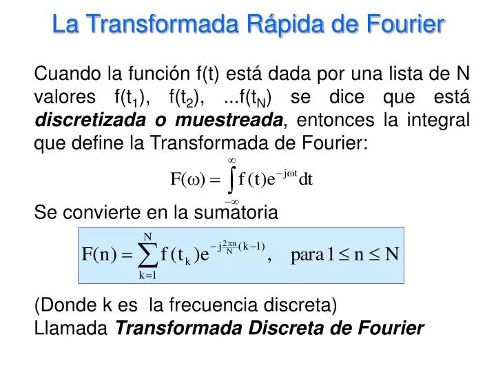
1. La Transformada Rápida de Fourier Cuando la función f(t) está dada por una lista de N valores f(t1), f(t2), ...f(tN) se dice que está discretizada o muestreada, entonces la integral que define la Transformada de Fourier: Se convierte en la sumatoria (Donde k es la frecuencia discreta) Llamada Transformada Discreta de Fourier

2. La Transformada Rápida de Fourier La Transformada Discreta de Fourier (DFT) requiere el cálculo de N funciones exponenciales para obtener F(n), lo cual resulta un esfuerzo de cálculo enorme para N grande. Se han desarrollado métodos que permiten ahorrar cálculos y evaluar de manera rápida la Transformada discreta, a estos métodos se les llama Transformada Rápida de Fourier (FFT)

3. f(t) 1 p . . . -T -T/2 0T/2 T . . . t -p/2 p/2 La FFT y la Serie de Fourier Podemos hacer uso de la FFT para calcular los coeficientes cn y c-n de la Serie compleja de Fourier como sigue: Ejemplo: Sea f(t) el tren de pulsos de ancho p y periodo T.

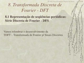
4. 32 muestras de f(t), de 0 a T 1.5 1 f(k) 0.5 0 0 1 2 k La FFT y la Serie de Fourier La versión muestreada f(k) de f(t) sólo puede tomar un número finito de puntos. Tomemos por ejemplo N=32 puntos cuidando que cubran el intervalo de 0 a T (con p=1, T=2):

5. La FFT y la Serie de Fourier Para obtener estas 32 muestras usando Matlab se puede hacer lo siguiente: k=0:31 f=[(k<8)|(k>23)] Plot(k,f,’o’)

6. La FFT y la Serie de Fourier Con los 32 puntos f(k) calculamos F(n) mediante la FFT, por ejemplo, en Matlab: F=fft(f)/N; Con lo que obtenemos 32 valores complejos de F(n). Estos valores son los coeficientes de la serie compleja ordenados como sigue:

7. La FFT y la Serie de Fourier Podemos graficar el espectro de amplitud reordenando previamente F(n) como sigue aux=F; F(1:16)=aux(17:32); F(17:32)=aux(1:16); F(n) queda: Y para graficar el espectro de amplitud: stem(abs(F)) Obteniéndose:

8. Espectro de Amplitud |F(n)| 0.6 Para el tren de pulsos p=1, T=2 |F(n)| 0.4 0.2 0 n 0 10 20 30 La FFT y la Serie de Fourier Si deseamos una escala horizontal en unidades de frecuencia (rad/seg):

9. Espectro de Amplitud |F(n)| 0.6 para el tren de pulsos, p=1,T=2 |F(w)| 0.4 0.2 0 w -50 0 50 La FFT y la Serie de Fourier w0=2*pi/T; n=-16:15; w=n*w0; Stem(w,abs(F)) Obteniendo:

10. La FFT y la Serie de Fourier También podemos obtener los coeficientes de la forma trigonométrica, recordando que: Podemos obtener Para el ejemplo se obtiene: a0=0.5, an=bn=0 (para n par), además para n impar:

11. 1 a0 0.5 Coeficientes an Coeficientes bn 0 -0.5 0 10 20 30 La FFT y la Serie de Fourier Como el tren de pulsos es una función par, se esperaba que bn=0; (el resultado obtenido es erróneo para bn, pero el error disminuye para N grande):

12. La FFT y la Serie de Fourier Tarea: Usar el siguiente código para generar 128 puntos de una función periódica con frecuencia fundamental w0=120p (60 hertz) y dos armónicos impares en el intervalo [0,T]: N=128; w0=120*pi; T=1/60; t=0:T/(N-1):T; f=sin(w0*t)+0.2*sin(3*w0*t)+0.1*sin(11*w0*t); Usando una función periódica diferente a la subrayada: a) Graficar la función. b) Obtener y graficar el espectro de amplitud de la señal usando la función FFT

13. Medidores Digitales La FFT ha hecho posible el desarrollo de equipo electrónico digital con la capacidad de cálculo de espectros de frecuencia para señales del mundo real, por ejemplo: • Osciloscopio digital Fuke 123 ($ 18,600.00 M.N.) • Osc. digital Tektronix THS720P ($3,796 dls) • Power Platform PP-4300

14. Medidores Digitales El Fluke 123 scope meter

15. Medidores Digitales Tektronix THS720P (osciloscopio digital)

16. Medidores Digitales Analizador de potencia PP-4300 Es un equipo especializado en monitoreo de la calidad de la energía: permite medición de 4 señales simultáneas (para sistemas trifásicos)

17. Fast Fourier Transform (FFT), I • DFT appears to be an O(N2) process. • Danielson and Lanczos; DFT of length N can be rewritten as the sum of two DFT of length N/2. • We can do the same reduction of Hk0 to the transform of its N/4 even-numbered input data and N/4 odd-numbered data. • For N = 2R, we can continue applying the reduction until we subdivide the data into the transforms of length 1. • For every pattern of log2N number of 0’s and 1’s, there is one-point transformation that is just one of the input number hn

18. Fast Fourier Transform (FFT), II • For N=8 • Since WN/2 = -1, Hk0 and Hk1 have period N/2, • Diagrammatically (butterfly), • There are N/2 butterflies for this stage of the FFT, and each butterfly requires one multiplication

19. Fast Fourier Transform (FFT), III • So far, • The splitting of {Hk} into two half-size DFTs can be repeated on Hk0 and Hk1 themselves,

20. Fast Fourier Transform (FFT), III • So far, • {Hk00} is the N/4-point DFT of {h0, h4,…, hN-4}, • {Hk01} is the N/4-point DFT of {h2, h6,…, hN-2}, • {Hk10} is the N/4-point DFT of {h1, h5,…, hN-3}, • {Hk11} is the N/4-point DFT of {h3, h7,…, hN-1}, • Note that there is a reversal of the last two digits in the binary expansions of the indices j in {hj}.

21. Fast Fourier Transform (FFT), IV

22. Fast Fourier Transform (FFT), V • If we continue with this process of halving the order of the DFTS, then after R=log2N stages, we reach where we are performing N one-point DFTs. • One-point DFT of the number hj is just the identity hj hj • Since the reversal of the order of the bits will continue, all bits in the binary expansion of j will be arranged in reverse order. • Therefore, to begin the FFT, one must first rearrange {hj} so it is listed in bit reverse order. • For each of the log2N stages, there are N/2 multiplications, hence there are (N/2)log2N multiplications needed for FFT. • Much less time than the (N-1)2 multiplications needed for a direct DFT calculation. • When N=1024, FFT=5120 multiplication, DFT=1,046,529  savings by a factor of almost 200.

23. Fast Fourier Transform (FFT), VI