Download
1 / 10
100 likes | 271 Views
Learning Scenario. The learner considers a set of candidate hypotheses H and attempts to find the most probable one h H, given the observed data. Such maximally probable hypothesis is called maximum a posteriori hypothesis ( MAP ); Bayes theorem can be used to compute it:.

E N D
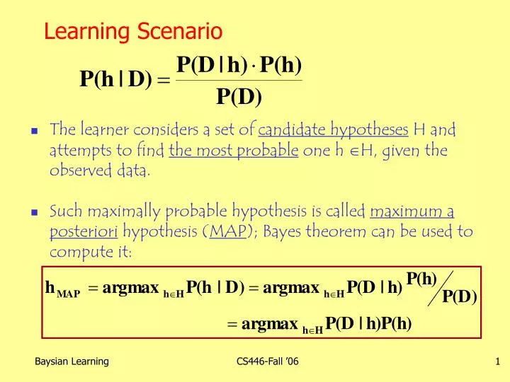
Learning Scenario • The learner considers a set of candidate hypotheses H and attempts to find the most probable one h H, given the observed data. • Such maximally probable hypothesis is called maximum a posteriori hypothesis (MAP); Bayes theorem can be used to compute it: CS446-Fall ’06
Learning Scenario (2) • If we ignore prior probabilities on H or assume all hypotheses are a priori equally probable • We get the Maximum Likelihood hypothesis: • This is the hypothesis that best explains the data without taking into account any prior preference over H CS446-Fall ’06
Examples • A given coin is either fair or has a 60% bias in favor of Head. • Decide which coin produced the data • Two hypotheses: h1: P(H)=0.5; h2: P(H)=0.6 • Prior: P(h): P(h1)=0.75 P(h2 )=0.25 • Now we need Data. 1stExperiment: coin toss is heads so D={H}. • P(D|h): P(D|h1)=0.5 ; P(D|h2) =0.6 • P(D): P(D)=P(D|h1)P(h1) + P(D|h2)P(h2 ) = 0.5 0.75 + 0.6 0.25 = 0.525 • P(h|D): P(h1|D) = P(D|h1)P(h1)/P(D) = 0.50.75/0.525 = 0.714 P(h2|D) = P(D|h2)P(h2)/P(D) = 0.60.25/0.525 = 0.286 CS446-Fall ’06
Examples(2) • A given coin is either fair or has a 60% bias in favor of Head. • Decide which coin produced the data • Two hypotheses: h1: P(H)=0.5; h2: P(H)=0.6 • Prior: P(h): P(h1)=0.75, P(h2)=0.25 • After 1st coin toss is H we still think that the coin is more likely to be fair • If we were to use Maximum Likelihood approach (i.e., assume equal priors) we would think otherwise. The data support the biased coin better. • Try: 100 coin tosses with 70 heads. • Now we will believe that the coins is biased: CS446-Fall ’06
Examples(2) • h1: P(H)=0.5; h2: P(H)=0.6 • Prior: P(h): P(h1)=0.75, P(h2)=0.25 • Experiment 2: 100 coin tosses; 70 heads. 0.0057 0.9943 CS446-Fall ’06
hML is often easier to find than hMAP • Recall • H is often parameterized or otherwise highly structured • hML can be found directly or iteratively from D • With prior information over H, Max P(h) < P(hML) • The difference Max P(h) – P(hML) allows other hH to be selected over hML to be hMAP • All of these must be examined CS446-Fall ’06
Parameterized Models • We attempt to model the underlying distribution D(x, y) or D(y | x) • To do that, we assume a model P(x, y | ) or P(y | x , ), where is the set of parameters of the model • Example: Probabilistic context-free grammars: • We assume a model of independent rules. Therefore, P(x, y | ) is the product of rule probabilities. • The parameters are rule probabilities. • Example: log-linear models • We assume a model of the form: P(x, y | ) = exp{(x,y) }/yexp{(x,y) } • where is a vector of parameters, (x,y) is a vector of features. CS446-Fall ’06
Log-Likelihood • We often look at the log-likelihood. Why? • Makes clearer / mathematically explicit that independence = linearity • Given training samples (xi; yi), maximize the log-likelihood • L() = i log P (xi; yi | ) or L() = i log P (yi | xi , )) • Monotonicity of log(.) means the that maximizes is the same CS446-Fall ’06
Parameterized Maximum Likelihood Estimate • Model: coin has a weighting “p” which determines its behavior: • Tossing the (p,1-p) coin m times yields k Heads, m-k Tails. • H is universe of p, say [0,1]. What is hML? • If p is the probability of Heads, the probability of the data observed is: P(D|p) = pk (1-p)m-k • The log Likelihood: L(p) = log P(D|p) = k log(p) + (m-k)log(1-p) • To maximize, set the derivative w.r.t. p equal to 0: dL(p)/dp = k/p – (m-k)/(1-p) • Solving this for p, gives: p=k/m (which is the sample average) • Notice we disregard any interesting prior over H (esp. striking at low m) CS446-Fall ’06
Justification • Assumption: Our selection of the model is good; that is, that there is some parameter setting * such that P(x, y | *) approximates D(x, y) • Define the maximum-likelihood estimates: ML = argmaxL() • Property of maximum-likelihood estimates: • As the training sample size goes to , then P(x, y | ML) converges to the best approximation of D(x, y) in the model space given the data CS446-Fall ’06