Download
1 / 10
130 likes | 488 Views
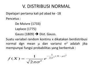
V. DISTRIBUSI NORMAL. Dipelajari pertama kali pd abad ke -18 Pencetus : De Moivre (1733) Laplace (1775) Gauss (1809) Dist. Gauss. Suatu variabel random kontinu x dikatakan berdistribusi normal dgn mean dan variansi 2 adalah jika mempunyai fungsi probabilitas yang berbentuk :.

E N D
V. DISTRIBUSI NORMAL Dipelajari pertama kali pd abad ke -18 Pencetus : De Moivre (1733) Laplace (1775) Gauss (1809) Dist. Gauss. Suatu variabel random kontinu x dikatakan berdistribusi normal dgn mean dan variansi 2 adalah jika mempunyai fungsi probabilitas yang berbentuk :
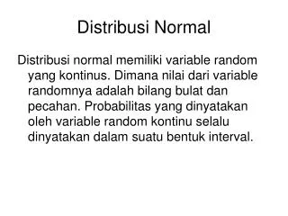
Untuk - < x < - < < 2 > 0 dan = 3,14 dan e = 2,718 Sifat-sifatdistribusi normal : • Harga modus, yaituhargapadasumbu x dengankurvamaksimumterletakpada x = • Kurva normal simetristerhadapsumbuvertikalmelalui • Kurva normal mempunyaititikbelokpada x = • Kurva normal memotongsumbumendatarsecaraasimtotis • Luasdaerahdibawahkurva normal dandiatassumbumendatarsamadengan 1.
Luas bagian kurva normal antara x=a dan x=b dapat ditulis menjadi P(a≤x≤b) Nilai ini untuk distribusi normal standar telah ditabelkan Tabel III Kurva normal : X Distribusi normal standar adalah distribusi normal yang mempunyai mean =0 dan standar deviasi =1 Untuk distribusi normal yang bukan distribusi normal standar maka diubah dengan rumus transformasi Z :
Tabel III. Distribusi Normal Nilaipadatabel III adalahluasdibawahkurva normal dari 0 sampaibilanganpositif b atau P(0≤Z≤b). Contoh : • Luaskurva normal dari 0 hingga 1,9 P(0 ≤ Z ≤ 1,9)=0,3621 KarenaKurva normal simetrisdi=0 maka P(-1,9 ≤ Z ≤0)= 0,321 Karenakurva normal simetrisdi=0 danluasdibawahkurva normal = 1 maka : P(0 ≤ Z ≤ +) = 0,5 dan P(-≤Z≤0)= 0,5 P(2,5 ≤ Z ≤ +) = 0,5 – P(0≤Z≤2,5)= 0,5 – 0,4798=0,0202 P(0,5 ≤ Z ≤ 2,5) = P(0 ≤ Z ≤ 2,5)- P(0 ≤ Z ≤ 0,5) = 0,4798 – 0,1915 =0,2883
2. Suatudistribusi normal mempunyai mean 60 danstandardeviasi 12. Hitunglah : • Luaskurva normal antara=60 dan x= 76 adalah : P(60 ≤ x ≤ 76) = …….. Dicaridulunilai Z-nya Jadi P(60 ≤ x ≤ 76)= P(0 ≤ Z ≤ 1,33) = 0,4082 • Luaskurva normal antara x1=68 dan x2=84. P(68 ≤ x ≤ 84)= P(0,67 ≤ Z ≤ 2,00)= 0,4772-0,2486 = 0,2284
Luaskurva normal antara x3=37 dan x4=72. P(37 ≤ x ≤ 72)= P(-1,92 ≤ Z ≤ 1,00) = P(-1,92 ≤ Z ≤ 0,00) + P(0,00 ≤ Z ≤ 1,00) = 0,4726 + 0,3412 = 0,8136 d. Luaskurva normal antara x4=72 sampaipositiftakterhingga P(72≤ x ≤ +)= 0,5 – P(0 ≤ Z ≤ 1,00) = 0,5 – 0,3412 = 0,1588
Contohaplikasidalambidang TP • Sebuahperusahaanmemproduksisusububukrendahlemak. Diasumsikankadarlemaksusububukmerk A berdistribusi normal dengan mean 3,5 % danstandardeviasi 0,3 %. • Berapakahprobabilitaskadarlemaksusububuk yang diambilsecaraacakberkisarantara 2,9 hingga 3,8 %? • Jikastandarpabrikmenentukanbahwamaksimalkadarlemaksusububuknyaadalah 4,0 %, hitunglahberapapersentaseproduk yang tidakmemenuhisyarattersebut?
Jawabansoalnomor 3. Diketahui : = 3,5 dan = 0,3 a. P( 2,9 ≤ x ≤ 3,8) = Sehingga : P( 2,9 ≤ x ≤ 3,8) = P( -2,0 ≤ x ≤ 1) = P( -2,0 ≤ x ≤ 0) +P( 0 ≤ x ≤ 1,0) = 0,4772 + 0,3412 = 0,8184 • P(X 4,0) = 0,5 – P(0≤ x ≤ 4,0) = 0,5 – P(0≤ Z ≤ 1,67) = 0,5 – 0,4525 = 0,0475
Pendekatan normal untuk binomial Distribusi normal akan memberikan pendekatan yang sangat baik jika n besar dan p mendekati 0,5. dalam hal ini : = np dan 2=np(1-p) sehingga : Contoh 4. Suatu proses produksi mempunyai kemungkinan 10% cacat, jika sampel sebanyak 100 buah diambil secara acak dari proses tersebut maka berapakah probabilitas : a. Delapan produk cacat b. Paling banyak lima produk cacat c. Paling sedikit lima belas produk cacat INGAT : Distribusi Normal : Kontinu VS Distribusi Binoamial : Diskrit
Jawab : Kejadian binomial tetapi n besarshgdidekatidengandistribusi normal, sehingga : = np = 100 X 10% = 10 2 = np(1-p) = 100. 10% X 0,9 = 9 = 3 Maka : • P(x = 8) = P (7,5≤ x ≤ 8,5) = P(-0,83 ≤ Z ≤ -0,5) = P (-0,83 ≤ Z ≤ 0) - (-0,5 ≤ Z ≤ 0) = 0,2967 – 0,1915 = 0,1052 b. P(x ≤ 5) = P(x ≤ 5,5) = P(Z ≤ -1,5) = 0,5 – P(-1,5 ≤ Z ≤ 0) = 0,5 – 0,4332 = 0,0668 c. P(x 15) = P(x 14,5) = 0,5 – P(0 ≤ x ≤ 14,5) = 0,5 – P(0≤ Z ≤ 1,5) = 0,5 - 0,4332 = 0,0668